In this post we discuss the algorithms we use to accurately recover implied dividend and interest rates from option markets.
Implied dividends and interest rates show up in a wide variety of applications:
- to link future-, call-, and put-prices together in a consistent market view
- de-noise market (closing) prices of options and futures and stabilize PnL’s of option books
- give tighter true bid-ask spreads based on parity and arbitrage relationships
- compute accurate implied volatility smiles and surfaces
- provide predictive models and trading strategies with signals based on implied dividends, and implied interest rate information
Data
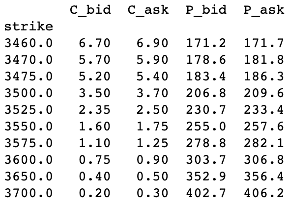
In order to recover implied dividends and interest rates from option prices we need bid-ask quotes for both calls and puts for a set of strikes. The options also need to be European-style. An example of such data is shown in the next table..
Preprocessing: fixing spreads
Working with real market data requires some pre-processing. An important check it to make sure that call and put spreads are non-negative. Call prices are by definition monotonic decreasing as a function of the strike, and for puts we have the opposite, monotonic increasing. This property holds independent of interest rates of dividends. Sometimes, real market option prices are not quotes as monotonic because there is no-one willing to offer to buy or sell a specific option for a competitive price. If that happens then anyone could in principle fix that by placing a bid or offer in the market without running any risk of being exposed to making a loss, and even potentially pick up a profit if someone decides to trade on your quote
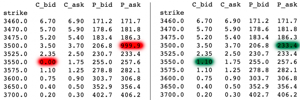
The table below gives two examples, shown in red, of quotes that break the monotonicity. The 3550 call bid quote of 0.00 can be increased to 1.10 (which is the bid of the next call with a higher strike),and the 3500 put offer of 999l0 can be lowered to 233.4. The logic goes as follows: if someone hits your 1.10 bid for 3550 call, you can then immediately sell the 3575 call for the same price of 1.10. In doing so you have bought a call-spread for free. Call spread can never have a negative value but they can potentially end up having a value as high at the difference in the two strikes (3575-3550=25).
The are in total 4 corrections we can do: check if we can increase the bids of both the calls and puts, and check if we can lower the offers of the calls and puts.
C_bid = np.maximum.accumulate(C_bid[::-1], axis=0)[::-1]
P_bid = np.maximum.accumulate(P_bid, axis=0)
C_ask = np.minimum.accumulate(C_ask, axis=0)
P_ask = np.minimum.accumulate(P_ask[::-1], axis=0)[::-1]
Besides having a minimum value, call and put spread also have a maximum value -the difference of the two strikes-. However, we can’t enforce this maximum with quote adjustments because this value will only materialise in the future on the options expiration date. This future payout makes todays maximum spread value interest rate dependent. We don’t know todays value of a future cashflow without knowing interest rates.
Call-Put parity: interest rates and dividends
To compute implied dividend and interest rates from option prices we need to utilize the call-put parity relationship. This parity relationship stems from the fact that buying a call and selling the put with the same strike will give you pay-off at the expiration date that is exactly like the stock -up to a constant shift-.
The figure below shows the payoff of the bought call option (in red), the payoff of the sold put option (in blue), and the combined payoff (in black). Both options have a strike of K=3250. If the stock reached 3400 on the expiration date then this option combination will be worth 150. If the stock S is at 3000 on the expiration date then this combination has a value -250.
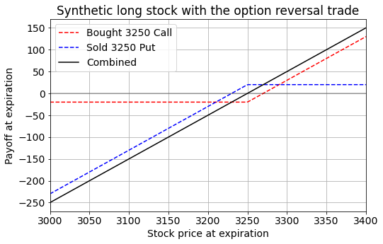
In general the payoff will be exactly S-K. This payoff can be turned into a “constant known guaranteed value” on the expiration date if we additionally sell the stock. Selling a stock today at S0 will give a payoff of S0-S at expiration. Combining this with the options’ payoff of S-K will result in a total payoff of S0-K, and this is independent of what the stock price S will be at expiration.
This “constant guaranteed value” forces a relationship on today’s call and put price. Buying a call for a price C and selling a put for a price P will cost C-P, and will always have a constant value of S0-K on the expiration date. This leads to a parity relation: C-P=S0-K.
The call-put parity formula has two extra elements. The first has to do with interest rates because we are talking about future payoffs. The second has to do will selling the stock. Having a long or short stocks position means that you might have to include dividend payment effects (if the stock gives a dividend somewhere before the expiration date). For European options on dividend-paying stocks, the put-call parity formula is given by:
![\[P-C=Ke^{-rt} - S0e^{-qt}\]](https://www.sitmo.com/wp-content/ql-cache/quicklatex.com-6cb3386954aff8d202995378a821d833_l3.png "Rendered by QuickLaTeX.com")
in this formula  are today’s call and put prices,
  the strike,
  the time to expiration in years,
  the continuously compounded interest rate,
  the current stock price, and
  the continuously compounded dividend yield.
Computing the bid & ask of synthetic underlying
The call-put-parity relation has 3 unknowns: C,P, and S0. If we know two of them we solve for the third. Since we have a table of call and put prices, we can thus compute the implied stock S0. Also, since the parity relationship involves buying and selling options on the bid and ask, we can compute a bid and ask price of the implied stock price.
For the synthetic dividend adjusted stock  we get:
(1) 
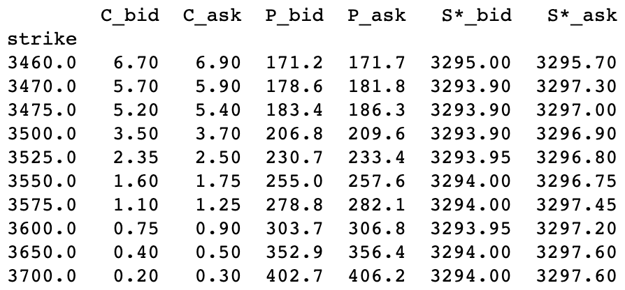
The synthetic dividend adjusted stock bid- and ask-prices are shown for a range of option strikes in the two rightmost columns in the table below. In this example we have simplified the calculation by assuming  . A key insight is that all these synthetic bid-ask quotes refer to the same synthetic underlying. Each strike gives us a bid-ask price for the same synthetic stock constructed from options with that strike. All these bids-ask prices should agree with one another, if not, then there will be an arbitrage opportunity. If one bid-ask range is outside the range of another then we can buy a synthetic underlying one way, and sell it another way, and make a guaranteed profit.
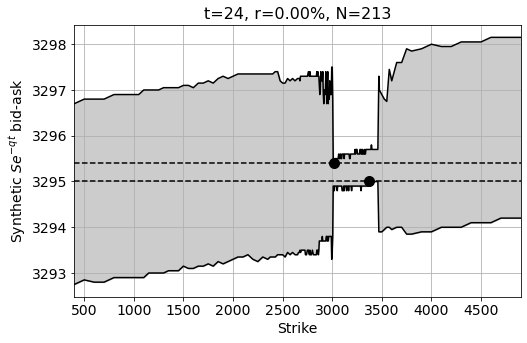
The plot below shows a diagram of all the bid-ask ranges for a large number of strikes. A typical feature is the narrower bid-ask spread for the liquid at-the-money options (in the strike range 3000-3500), and wider bid-ask ranges for the illiquid out-of-the-money options. Liquidity of he options is one reason for tight/wide spreads, and another reason is that for out-of-the-money strikes, either one of the call or put will always have a large delta. A high delta which makes the option price very sensitive to changes in the underlying, and since the underlying is volatile this will case bid-ask ranges to widen.
The plot also shows the best-bid and best-offer (dashed lines). If you would want to sell the synthetic underlying they you will get the highest price by selling it using the options with strike=3400 (black dot on the bottom dashed line).
A third thing to note is that the bid-ask ranges show an upward trend as a function of the strike. This is because we have simplified the calculation by assuming interest rates r to be zero -which is apparently wrong-. Looking back at the above equations we can see that changing r affects the contribution of K. By increasing or decreasing r we can change slope. If we change it the wrong way we can cause the highest-bid to rise above the lowest offer, and that would give rise to an arbitrage opportunity. This is unlikely to happend in the tradable market, and this would be a good indication that the interest rate we’ve used in our calculations is a wrong one. Taking this further, we can estimate the implied interest rate used in the market through optimisation.
Estimating implied interest Rates with least squares regression
A very efficient and elegant way to estimate an implied interest rate is through least squarers regression. I was first pointed out to this fact by Alan Lewis when we were brainstorming about his “Option-based Equity Risk Premiums” project. The call-put parity relation:
![\[P-C=Ke^{-rt} - Se^{-qt}\]](https://www.sitmo.com/wp-content/ql-cache/quicklatex.com-c3979aa08322a0ddaf2357c8bfa4cb1a_l3.png "Rendered by QuickLaTeX.com")
can be seen as a linear equation, linear as a function of the strike K:
![\[y = K a +b\]](https://www.sitmo.com/wp-content/ql-cache/quicklatex.com-fa6ccca6a3dd44e6a8462fd2f7657ac9_l3.png "Rendered by QuickLaTeX.com")
with
 . In this form we can estimate
  and
and  with ordinary least squares regression. When computing
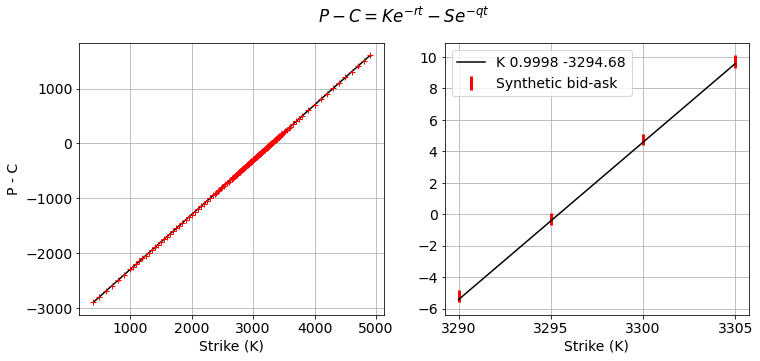
  we pick the mid market values of the calls and puts. The regression formulation is plotted below. On the left you see a full range on quotes based on mid market prices, and on the right a detail zoom where we have also plotted the bid-ask range around those y-values.
The regression gives us  and
and  .
.
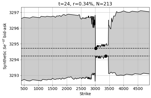
The plot below shows the range plot for  , as you can see most of the tilt has gone.
Note 1: there is also an alternative linear formulation that can also be used (eq. 17 in Alan’s paper)
![\[\frac{P-C}{K} = e^{-rt} + \left(\frac{S0}{K}\right)e^{-qt}\]](https://www.sitmo.com/wp-content/ql-cache/quicklatex.com-119b450c3ae0c69fc8d51193672985c7_l3.png "Rendered by QuickLaTeX.com")
This can be seen as an alternative weighted version of the previous equation. In this alternative formulation all the data-points give a weight of  to
to  (was ) and a weight of
  to
to  (was ). Effectively this shifts importance away from high strikes and makes low strikes equally important as high strikes.
Note 2: the regression estimates values for  ,and from this we can compute
  . If one of
  unbiased then the other is not due to the non-linear mapping between them. In practice this is neglect-able in the context of other uncertainties.
Estimating implied interest rate with bid-ask range overlap optimization
Even though least-squares fitting on the mid prices gives a good fit (and also does that fast), it has shortcomings. First, the least-squares objective doesn’t have a clear financial meaning like an “arbitrage constraint” or a “parity rule”. Second, the solution is sensitive to bid-ask spread adjustment, every individual single bid-ask change will change the least-squares solution, and ideally we would like to have a solution that’s less sensitive.
An alternative objective when looking for an optimal interest rate is to maximize the amount of agreement between all the bid-ask spread of the synthetic underlying, and especially make sure that there is no disagreement. If bid-ask spread disagrees then this means that there is an arbitrage opportunity: one can buy a synthetic underlying using the options of one strike, sell the synthetic underlying using options of a different strike. In our optimization we will look at two things: minimize the number of arbitrage opportunities, and maximize the total amount of agreement across all possibilities pairs of synthetic underlyings.
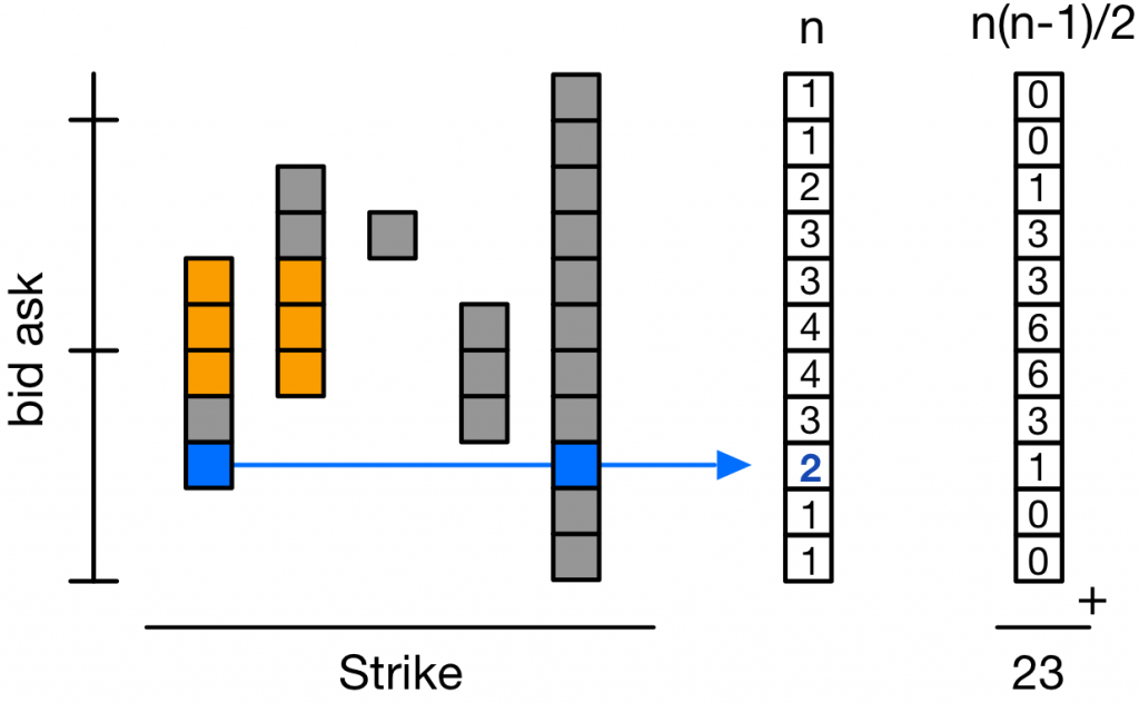
Efficient computation of the total mutual bid-ask range overlap
In the example plot below we have 5 bid-ask ranges for 5 synthetic underlying for 5 different strikes. The first two strikes (K1,K2) have a mutual overlap of 3 (orange regions). If we look at all possible pair combinations we have: (K1,K2) 3, (K1,K3) 0, (K1,K4) 3, (K1,K5) 5, (K2,K3) 1, (K2,K4) 2, (K2,K5) 5, (K3,K4) 0, (K3,K5) 1, and(K4,K5) 3. The total mutual range overlap is thus 3+0+3+5+1+2+5+0+1+3 = 23. Computing the total mutual range overlap by iterating over all possible pairs is an  algorithm (with
  the number of ranges), which is inefficient.
The total range overlap can be computed in  using the following algorithm. The algorithm starts by computing the counts
  of how many times a bucket is covered by all ranges. E.g. the bucket count for the bucket next to the blue arrow is “2” because there are two ranges that (K1, K5) that intersect with this bucket (the blue squares). Computing these counts can be done in by looping over the strikes, and for each strike incrementing the range of buckets that overlap with that strike. Once all strikes are processed, we can compute the total mutual range overlap by summing the
  values.
def sum_mutual_overlap(bids, asks, width=0.1):

    first_bin = int(min(bids)/width)
    last_bin = int(max(asks)/width)

    n = np.zeros(last_bin - first_bin + 1, dtype=np.int32)

    for bid, ask in zip(bids, asks):
        start = int(bid/width) - first_bin
        stop = int(ask/width) - first_bin

        n[start:stop+1] += 1

    return width * np.sum(n*(n-1)/2)
Computing the number of arbitrage opportunities
There is an arbitrage opportunity whenever the bid-ask range of one synthetic underlying is outside the bid-ask range of a second bid-ask range. Counting the number of arbitrage opportunities can also be done with an algorithm by keeping a running count of the bid and ask distributions while looping over the strikes.
def count_arb_violations(bids, asks, width=0.1):

    first_bin = int(min(bids)/width) - 1
    last_bin = int(max(asks)/width) + 2

    n_bids = np.zeros(last_bin - first_bin + 1, dtype=np.int32)
    n_asks = np.zeros(last_bin - first_bin + 1, dtype=np.int32)

    num_arbs = 0
    for bid, ask in zip(bids, asks):
        bid_bin = int(bid/width) - first_bin
        ask_bin = int(ask/width) - first_bin

        num_arbs += np.sum(n_asks[:bid_bin]) + np.sum(n_bids[ask_bin+1:])

        n_bids[bid_bin] += 1
        n_asks[ask_bin] += 1

    return num_arbs
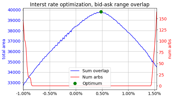
Finding the optimal implied interest rate is done by looping over a range of trial interest rates, and picking the interest rate value that has the highest tot range overlap in the region with the lowest number of arbitrage counts. The plot below shows the result of the optimization. All interest rate values in the range [-0.8%, +1.4%] result in zero arbitrage opportunities. Inside that zero arbitrage region, the total area peaks for an interest rate of 0.48%.
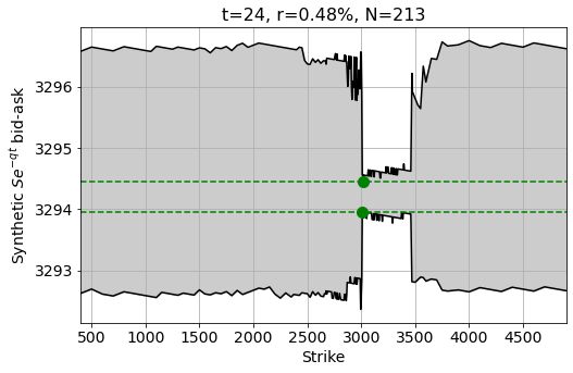
The plot below shows the bid-ask ranges of the optimal implied interest rate of 0.48%. Compared to the least-squares fit we see that there is less tilt in the range diagram, and we also know that this solution is arb free. The green lines are the highest bid and lowest ask.
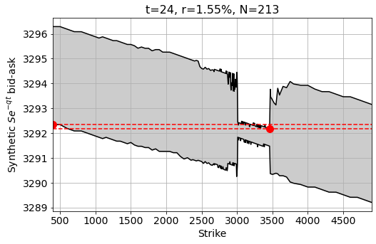
Below an example of an interest rate choice of r=1.55% that gives rise to arbitrage. The highest bid of the synthetic underlying (the leftmost value of the bottom of the region K=400) is higher than the lowest offer of the same synthetic underlying (lowest value of the top line of the region K=3500).
Implied dividend yield
Once we have estimated the optimal implied interest rate, we also have an estimate of the best bid and ask of the synthetic dividend adjusted stock price  . This value has two unknowns, the dividend yield that we are looking for, and the current stock price. A good estimate of the current stock price S0 can be gotten from the synthetic underlying based on option prices with the shortest time till expiration. When is small, then will be close to 1 for typical values of (a typical value for q is 2%),and hence
  .
.
Results
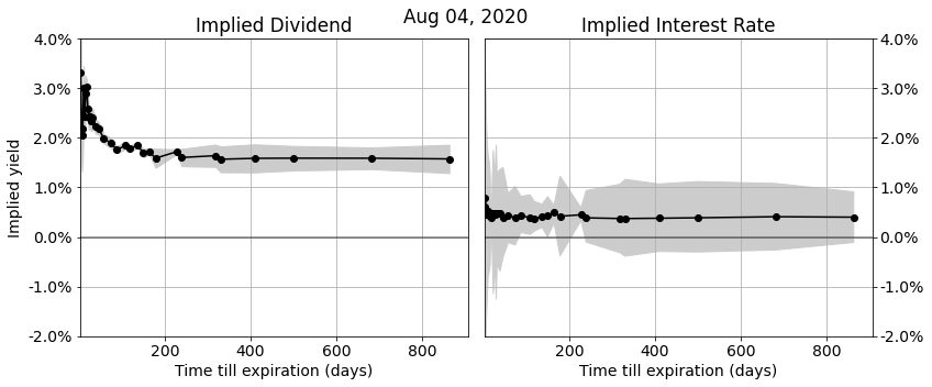
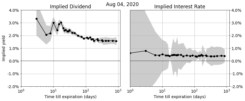
So far we have discussed computing the implied interest rate and dividend yield for a single option expiration series. Repeating the same calculation for all option expirations gives an implied dividend and interest rate term structure. The plots below show the implied dividend and interest rate terms structures for the S&P500 options on Aug 4, 2020. The black lines show the optimal fits, the grey regions show the no-arbitrage bounds. The horizontal time-axis is linear in the top plot, and logarithmic in the bottom plot.
In follow-up posts we will:
- look at the time evolution of these implied terms structures
- move on to modeling implied volatility smiles and surfaces