Extracting Interest Rate Bounds from Option Prices – SITMO Machine Learning

In this post we describe a nice algorithm for computing implied interest rates upper- and lower-bounds from European option quotes. These bounds tell you what the highest and lowest effective interest rates are that you can get by depositing or borrowing risk-free money through combinations of option trades. Knowing these bounds allows you to do two things:

1. Compare implied interest rate levels in the option markets with other interest rate markets. If they don’t align then you do a combination of option trades to capture the difference.

2. Check if the best borrowing rate is higher than the lowest deposit rate. If this is not the case, then this means there is a tradable arbitrage opportunity in the market: you can trader a combination of options that effectively boils down to borrowing money at a certain rate, and at the same time depositing that money at a higher rate.

In practice we won’t see these types of tradable arbitrage opportunities a lot in live markets, however, there is two important applications for doing this analysis:

Market data reports typically combine market data from different sources, or combine snapshots of the market at slight different points in time, and because of this option prices are noisy and often inaccurate. Option price quotes needs to be checked and corrected in order to have a clearer view on the true market prices. Clear prices help us calibrate option pricing models better, and hence give us better greeks for hedging our option positions and tracking the PnL of our option books.
Implied interest rate in option prices tells us something about the sentiment in option markets. This sentiment can be a valuable input for trading trategies.

Synthetic stocks from option quotes, and arbitrage conditions

The next plot shows a snapshot of SPX options prices as the close of Jan 24, 2020. The prices are for options that expire on Feb. 21, 2020:

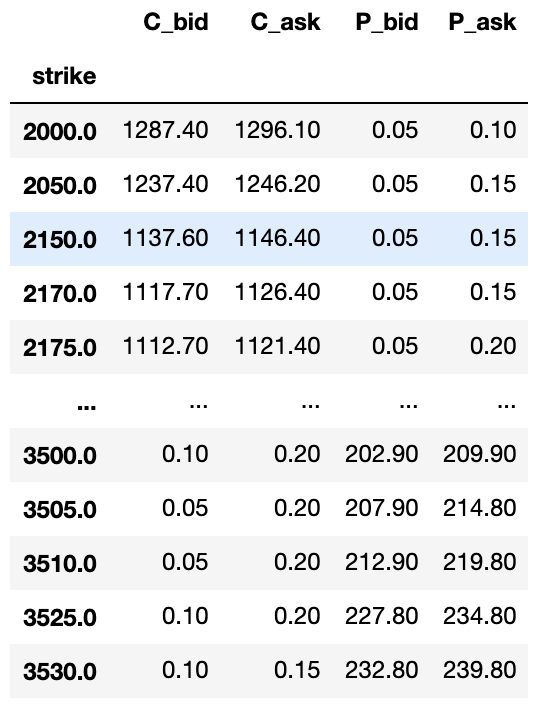
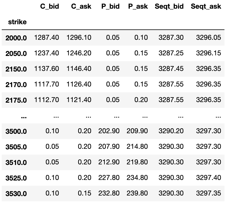
We can buy a synthetic long stock by buying a call and selling the put with the same strike. E.g. for the 2000 strike we can buy the call for 1296.10 (at the call’s ask price) and sell the put for 0.05 (at the put’s bid price). Combined we have paid 1296.05, and we know from theory that the value of this combination will be S-2000 at expiration. This gives us a good indication of what S might be: if you invest 1296.05 and expect to receive S-2000, then this investment would only make a profit if S > 1296.05 + 2000 = 3296.05. Similarly, we can also do the opposite trade, sell a synthetic stock by selling a call at 1287.40 and buying a put at 0.10. This sold synthetic stock will only make a profit if a<3287.30. The table below shows the synthetic long and short prices in the two rightmost columns for all strikes.

It would have been awesome if we could have bought a synthetic stock at some price and sell the synthetic stock at a higher price, and make a guaranteed profit. Unfortunately in this case using the 2000 strike options we would buy the synthetic stock at 3296.50 and sell it lower at 3287.30, and have a guaranteed LOSS of 8.75. The loss is easy to explain because we both buy and sell the call and put option, losing the bid-ask spread (8.70 for the call, 0.05 for the put).

We are however not limited to buying and selling the synthetic stock using options of all the same strike. E.g. we can but the synthetic stock for 3296.05 using the options with strike 2000, and sell the synthetic stock for 3290.30 using options with strike 3505. This gives us a loss of 5.65, which is substantially better than the earlier 8.70 loss.

This leads us to a simple strategy for searching for an arbitrage strategy. We will have found an arbitrage opportunity if the lowest price we can buy a synthetic stock for (lowest value in the rightmost column) is below the highest values we can sell the synthetic stock for (highest values in the 2nd last column).

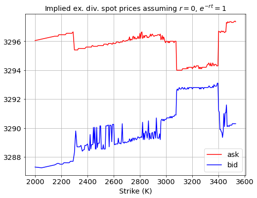
The figure below shows a plot of the bid- and ask-price of synthetic stock for the various strikes. It’s easy to see that there is no arbitrage opportunity: the highest bid (highest point on the blue line, somewhere around the 3400 strike) is below the lowest ask price (lowest value on the red curve, somewhere around the 3100 strike).

Interest rate effects

There are two more ingredients we need to add: the value of the synthetic stock is S-K is a value at expiration, which is at some future point in time. Today’s value would be different due to interest rate effects and dividend effects. The full synthetic stock price formulate is:

$S(K)e^{-qt} = C(K) - P(K) +Ke^{-rt}$

$q$ here is the dividend yield, and it accounts for the fact that getting a stock in the future instead of today means that you might be missing out on upcoming dividend payments. $r$ is the interest rate, and $t$ the time till expiration.

Dividends and interest rates have different effects: dividends cause an absolute shift in the left-hand-side, whereas interest rates have an effect that depends on the value of the strike: the term $Ke^{-rt}$ shows that the interest rate effect $e^{-rt}$ gets scaled up by the size of the strike $K$ .

The bid-ask curves in the plot above were computed by setting that interest rate to zero. If instead we would pick a different value such that $e^{-rt}=0.99$ , then the plot will look like this:

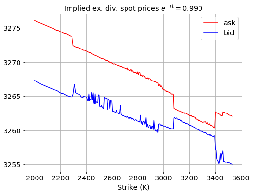
This plot DOES show arbitrate opportunities: we can buy the synthetic stock for 3261 using options with strike 3400 and sell the synthetic stock higher at 3267 using options with strike 2000. In reality, such an easy arbitrage opportunity will never happen, and so it’s very likely that our $e^{-rt}=0.99$ is wrong. If our value is right then that would imply that there are lots of real, tradable, arbitrage opportunities in the market.

This leads us to “implied interest rate bounds” based on arbitrage opportunities. what interest rate values are sensible, assuming that the market is not dumb enough to offer free arbitrage?

Separating common tangents

Interest rates change the slope of the bid-ask curve, and we introduce arbitrage if the highest value of the bottom curve exceeds the lowest value of the top curve. By changing the interest rate parameter we can search for bounds, find the interest rate values that cause the highest bid to exactly match the lowest ask, and further tilting would cause an arbitrage. Rather than a brute force search and trying many test values, we can use a more elegant and faster algorithm based on the paper “Common Tangents of Two Disjoint Polygons in Linear Time and Constant Workspace” Abrahmses, M. et al. 2018, doi:10.11245/3284355.

It can be shown that finding the maximum tilts is equivalent to finding the slopes of “separating common tangents” between the bid and ask curve. The concept of separating common targets is shown in the figure below (taken from the paper).

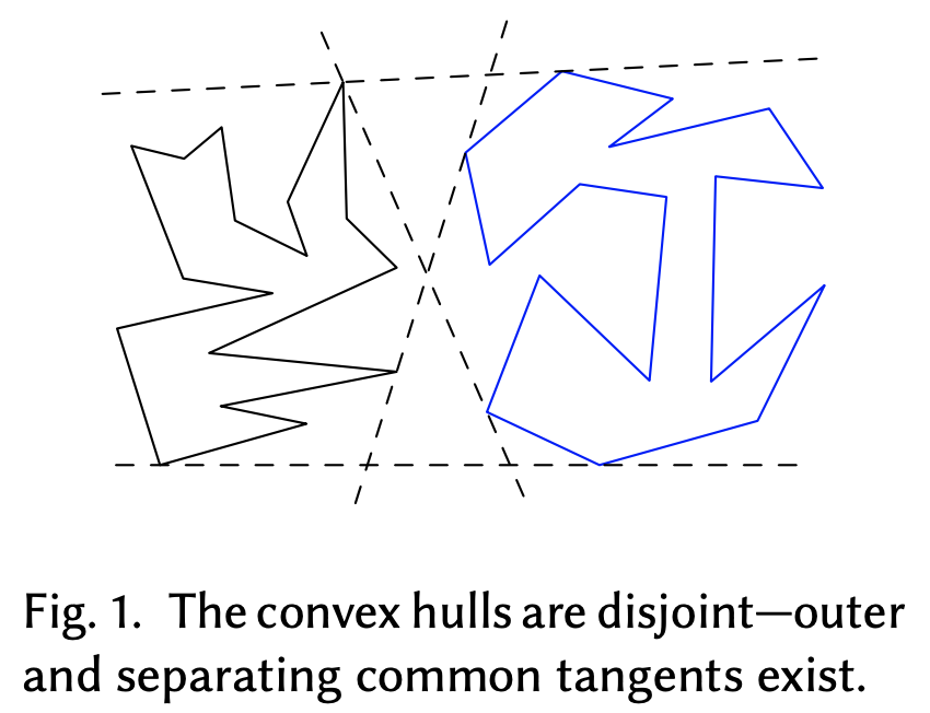
The separating common tangents are the two dashed lines in the middle that cross one another. These lines are the steepest possible lines that fit inside the gap between the two polygons. Both tangents tough both polygons exactly once.

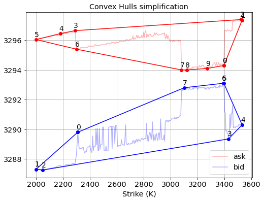
Convex Hull packing

Although not necessary, we first compute the convex hulls of the bid and ask curves and apply the common tangent search algorithm to the convex hulls instead of the original bid-ask curves. The purpose of this step is to reduce the number of data points that the algorithm needs to work on. Working with the full bid- and ask-curve or with the convex hulls of those curves gives the exact same solution. The convex hull can be computed very fast with scipy.spatial library, and it reduces the number of data points with a factor 10-100.

from scipy.spatial import ConvexHull

ask_hull = ConvexHull(ask_points)
bid_hull = ConvexHull(bid_points)

The algorithm is quite simple as is illustrated below.

First, pick two random points -one on each of the hulls-, and connect them with a line (dashed line), this is called the “candidate line”.
Next, move counterclockwise along the hull and check if the new point is on the correct side of the line. In this example, we want to find the common tangent that has the red ask curve on the LEFT, and the blue bid curve on its RIGHT. The new point is on the wrong side of the line, and hence we move the candidate line to point to this new point.

this process is repeated, alternating between the upper- and lower-hull.

At some stage, all point on both sides will be on the correct side of the tangent, and this gives the final solution. The algorithm stops when the candidate line hasn’t changed for a full sweep of all points on both sides.

An important element of this algorithm is to test if a point is left or right of a given line. In the plot below the point “p” is left of the line “a->b”. One way to test that is by computing the determinant of the two vectors “a->p” and “a->b”. The determinant is basically the area that is spanned by the two vectors (blue rhombus), but the sign of the determinant depends on the point “p” being on the left or right.

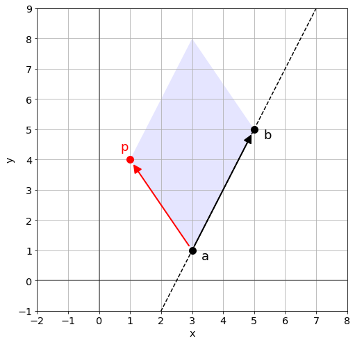
a = np.array((3,1))
b = np.array((5,5))
p = np.array((1,4))

m = np.column_stack((p-a, b-a))

d = np.linalg.det(m)

print(d)
> -14   # negative means "p is left of a->b"

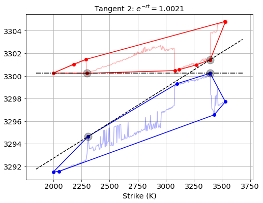
Running the common tangents algorithm on the convex hulls of the bid and ask curves give the following result:

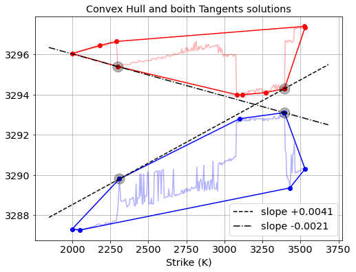
The slopes of the two computed tangents can now be used to find bounds on the $e^{-rt}$ strike slope factor. The highest “valid interest rate” is for $e^{-rt}=0.9959$

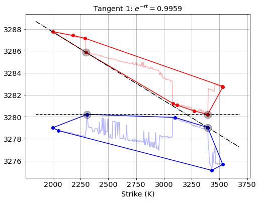
… and the lowest valid interest rate is for $e^{-rt}=1.0021$ .

Outlier detection

A final note:

The common tangents algorithms can end up telling you that there is “no solution”, if this happens then that means that the two convex hulls overlap and that there is arbitrage opportunity in the market no matter what the true interest rate is!

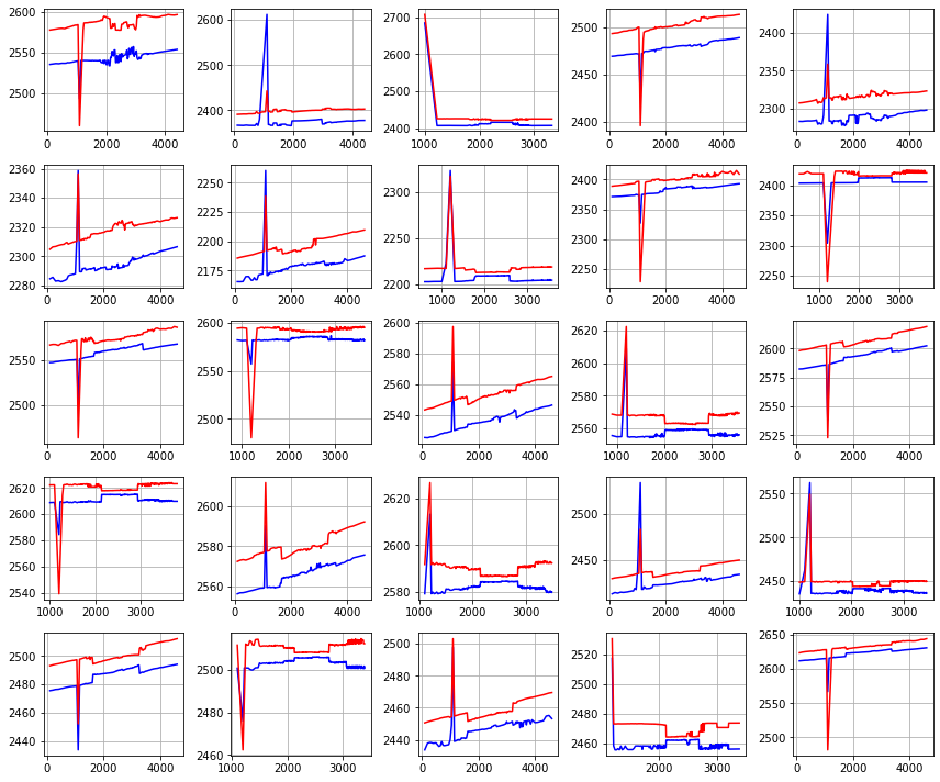
Below a set of 25 plots of arbitrage opportunities found in our raw market data feed. For the SPX options series we see outliers like this once every 2 days. If left untreated then these misprints will cause trouble in market-to-market valuation, model calibration steps, and hedges. Most of these arb opportunities are non-tradable, misprints of flawed quotes. In a follow-up post we will discuss a robust algorithm to remove these outliers.

By : Thijs van den Berg