Back-testing trading strategies is a dangerous business because there is a high risk you will keep tweaking your trading strategy model to make the back-test results better. When you do so, you’ll find out that after tweaking you have actually worsened the ‘live’ performance later on. The reason is that you’ve been overfitting your trading model to your back-test data through selection bias.
In this post we will use two techniques that help quantify and monitor the statistical significance of backtesting and tweaking:
- First, we analyze the performance of backtest results by comparing them against random trading strategies that similar trading characteristics (time period, number of trades, long/short ratio). This quantifies specifically how “special” the timing of the trading strategy is while keeping all other things equal (like the trends, volatility, return distribution, and patterns in the traded asset).
- Second, we analyse the impact and cost of tweaking strategies by comparing it against doing the same thing with random strategies. This allows us to see if improvements are significant, or simply what one would expect when picking the best strategy from a set of multiple variants.
Stock Data
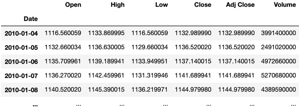
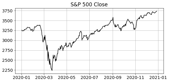
To illustrate these techniques, we downloaded a csv with a couple of years of historical daily S&P500 price data from yahoo finance, save it to disk, and then read it with pandas:
import pandas as pd
data = pd.read_csv('GSPC.csv', index_col=[0], parse_dates=True)
Trading Strategy
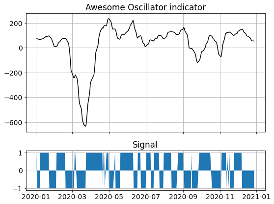
Next, we are going to test a simple trading strategy that is based on the Awesome Oscillator indicator from the Python Technical Analysis library. We picked this indicator purely because of its promising name, we have not looked at what it’s doing exactly (on purpose).
import ta

ind = ta.momentum.AwesomeOscillatorIndicator(data.High, data.Low).awesome_oscillator()
Using this indicator, a simple trading strategy would be to be buy the S&P when the indicator is going up, and sell the S&P (short) when the indicator goes down:
import numpy as np

signal = np.sign(ind.diff(1))
Performance Measurement
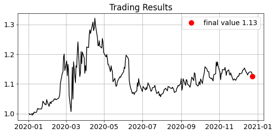
The performance time series of this strategy is easily computed by compounding day-ahead returns that are multiplied by the signal sign. If the indicator is higher today than it was yesterday we will buy at today’s close and go long. Depending on what the S&P index will do tomorrow this will be a good trade or not. For simplicity we assume we can trade every day at the Close, without transaction costs.
There is of course other performance metrics (like Sharpe Ratio) that one could use, the concepts in this article are generic and not tied to any specific performance metric.
v = np.cumprod(1 + (signal * data.Close.pct_change().shift(-1)))
Generating Random Strategies with Markov Chains
To test how special the Awesome Generator performance is, we can compare it against random strategies, and see if the performance is significantly better than most of those the random strategies.
When we do this, it’s important to compare apples with apples. The random strategies need to look similar to the strategy we are testing. If they don’t and e.g. had a very different long / short ratio (the fractions of times that the strategy is long or short), or a very different trading frequency (number of trades per year), then the comparison would be unfair due to factors like transaction costs, or behavioral aspects like whether the market is always going up (or not).
A good choice is to make sure that the random strategies have a similar long / short ratio, and a similar number of trades, and only differ in the timing of when they switch from long to short and back. This will result in a comparison that focuses on the quality of the timing of the strategy and exclude the effects of other factors.
On average, the Awesome Oscillator seems to be long / short half of the time.
signal.value_counts()
>
 1.0    128
-1.0    122
One could thus generate a simple comparable random strategy with a coin-flip simulation that randomly pick either a signal value if -1 (short) or +1 (long).
np.random.choice([1,-1], size=10)

> array([ 1,  1,  1, -1, -1,  1, -1,  1, -1, -1])
Even though this will result in a strategy that’s on average long / short half of the time, it will however also flip signs 50% of the times, -i.e. trade 50% of the days-. The Awesome Oscillator on the other hand shows a more ‘sticky’ behavior: when long, it is often again long the next day, in this case historically 84% of the time. This is significantly different than the 50% we get with Python’s random choice.
The code below shows how to analyze this sticky behavior. First we create a Panda’s DataFrame with two column: the current state (long/short) and the next day’s state, and then we create a pivot_table that counts the number of times we’ve seen various combinations of long / short positions from one day to the next.
twoday = pd.DataFrame({'cur':signal, 'next':signal.shift(-1)})
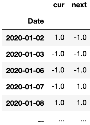
trans_count = twoday.pivot_table(index='cur', columns='next', aggfunc='size', fill_value=0)
Using these “current vs next day”‘s state counts, we can now compute the state transition probabilities. This probability matrix has for each row (current state) the probabilities of going to the next state (columns). This matrix is known as the Stochastic Matrix.
trans_prob = trans_count.div(trans_count.sum(axis=1), axis=0)
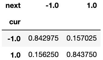
In this matrix we see in the bottom left corner that there is a 0.16250 probability that we switch from a long position (1.0 row label) to a short position (-1.0 column label) in the next day. The Stochastic Matrix is often visualised with a state transition diagram like below.
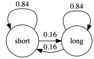
A state transition model like this is called a Markov Chain, and we will use the the transition matrix to generate random state transition sequences with code like below:
current_state = -1
for _ in range(10):
    current_state = np.random.choice(trans_prob.columns, p=trans_prob.loc[current_state])
    print(current_state)

>
1.0
1.0
1.0
1.0
1.0
1.0
1.0
-1.0
-1.0
-1.0
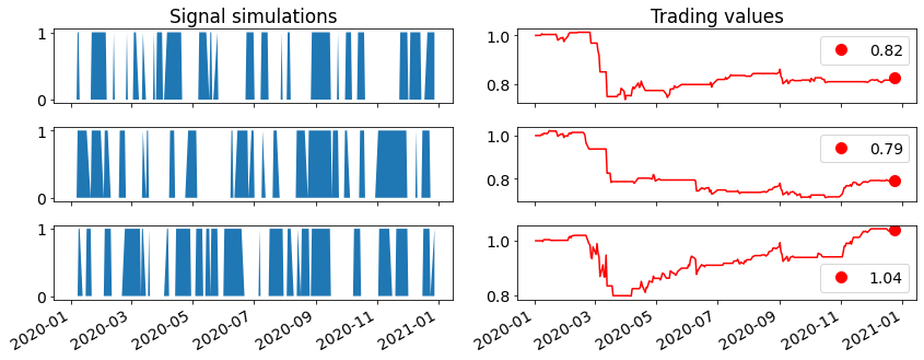
Below is a plot with on the left three random scenarios generated with this Markov Chain transition matrix model, and the trading results of those scenarios on the right. The idea is that these random trading scenarios have similar characteristics as the Awesome Oscillator, except that the timing is purely random and not based on any market information.
Simulation results
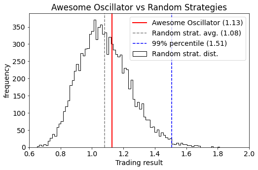
The next plot show results based on 10.000 random trading scenarios. The performance distribution of the random strategies is shown in black, and we see that the Awesome Oscillator (in red) is somewhere in the middle of the distribution. This is telling us that the Awesome Oscillator is not any better than random strategies. A good strategy that is statistically significantly better than a random strategy would have had a performance above the 99% percentile (to the right of the blue line).
Searching for better strategies
If we read the manual of the Awesome Oscillator, we see that it has two magic numbers {window1, window2} that we can change. We can try to change those, and see if that gives us a better performing strategy.

Suppose we try 10 different settings and then pick the best one: surely we will end up with a better strategy? The probability that all 9 new variants are all worse is very low.
But, what if we instead considered 9 alternative random strategies? There is a high likelihood that in that case one of the random strategies would be best! However, this is NOT something we want, we don’t want to discard our strategy and replace it with a random strategy, because a random strategy is not something we want to actually trade on.
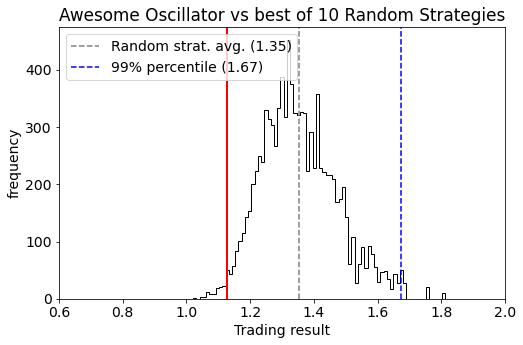
This brings us to the main point: if you try multiple strategies and pick the best one, then you need to benchmark that selection process against picking the best of multiple random strategies. Below you see the distribution of the performance of “best-of-10” random strategies. Compared to a single random strategy, the “best-of-10” has a higher mean (now 1.35 vs 1.08 previously), and a higher significance level (now 1.67 vs 1.51 previously). If we look at 10 strategy backtests during our research and pick the best one, then it will only be something you can put to production if the performance is about 1.67. Anything below is not statistically significantly better than putting random strategies to production.
There is one subtle factor to look into: if your strategies are all very similar (which is often the case when tweaking) then it’s not fair to treat them as independent separate strategies. Maybe 10 variants of a strategy only count effectively as 2 very different strategies because they are all very much alike?
Another thing to note is that having a separate train and validation set isn’t going to help unless you don’t look at the validation performance when deciding what strategy you’ll eventually pick.
For further reading: Marcos Lopez de Prado has done extensive research on backtesting and these biases. I highly recommend his books and his research on the “Deflated Sharpe Ratio”.