Category: Statistics (Page 1 of 2)

Forecasting Current Market Turbulence with the GJR-GARCH Model

April 6, 2025 / Thijs van den Berg

The Current Market Shake-Up

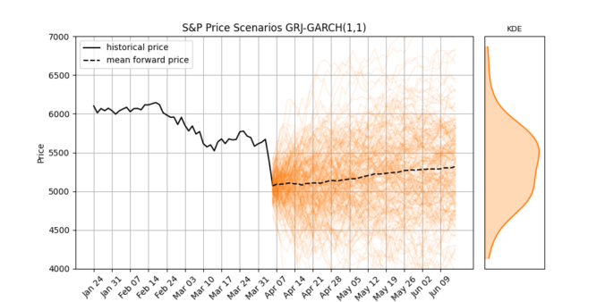
Last week, global stock markets faced a sharp and sudden correction. The S&P 500 dropped 10% in just two trading days, its worst weekly since the Covid crash 5 years ago.

Big drops like this remind us that market volatility isn’t random, it tends to stick around once it starts. When markets fall sharply, that volatility often continues for days or even weeks. And importantly, negative returns usually lead to bigger increases in volatility than positive returns do. This behavior is called asymmetry, and it’s something that simple models don’t handle very well.

In this post, we’ll explore the Glosten-Jagannathan-Runkle GARCH model (GJR-GARCH), a widely-used asymmetric volatility model. We’ll apply it to real S&P 500 data, simulate future price and volatility scenarios, and interpret what it tells us about market expectations.

Using Fractional Brownian Motion in Finance: Simulation, Calibration, Prediction and Real World Examples

April 5, 2025 / Thijs van den Berg

Long Memory in Financial Time Series

In finance, it is common to model asset prices and volatility using stochastic processes that assume independent increments, such as geometric Brownian motion. However, empirical observations suggest that many financial time series exhibit long memory or persistence. For example, volatility shocks can persist over extended periods, and high-frequency order flow often displays non-negligible autocorrelation. To capture such behavior, fractional Brownian motion (fBm) introduces a flexible framework where the memory of the process is governed by a single parameter: the Hurst exponent.

The Visible Shape of Random Galaxies: What You Get When You Project a 3D Disk

March 31, 2025 / Thijs van den Berg

When we look at galaxies through a telescope, we see them as ellipses. But real galaxies are 3D disks randomly oriented in space. This post shows how we can simulate that: we start with a random orientation, project a flat disk into the 2D image plane, and extract the observed ellipse parameters. This setup helps us understand what shape distributions we expect to see in the absence of structures like gravitational lensing and clustering.

In research we can analyse and compare the properties of this pure random reference model against real observations to look for subtle distortions

How to Sample the 3D Universe You See in an Image

March 31, 2025 / Thijs van den Berg

When we look at an astronomical image, we see a 2D projection of a 3D universe. But suppose we want to simulate the distribution of galaxies behind that image, for example, to generate synthetic data, test detection algorithms, or check if real galaxy distributions statistically deviate from what we’d expect under uniformity. To do this, we need a way to sample galaxies uniformly in 3D space, restricted to the cone of space visible in an image.

The Odds of Outshining: When One Coin Beats Another

March 25, 2025 / Thijs van den Berg

Imagine you’re comparing two trading strategies. One has made a handful of successful trades over the past month, while the other shows a different success pattern over a slightly shorter period. Both show promise, but which one truly performs better? And more importantly, how confident can we be in that judgment, given such limited data?

To explore this, let’s turn to a simpler but mathematically equivalent situation: comparing two coins. The first coin is flipped 10 times and lands heads 3 times. The second coin is flipped 9 times and lands heads 5 times. We want to know: what is the probability that the second coin has a higher chance of landing heads than the first?

Yield Curve Interpolation with Gaussian Processes: A Probabilistic Perspective

March 23, 2025 / Thijs van den Berg

Here we present a yield curve interpolation method, one that’s based on conditioning a stochastic model on a set of market yields. The concept is closely related to a Brownian bridge where you generate scenario according to an SDE, but with the extra condition that the start and end of the scenario’s must have certain values. In this paper we use Gaussian process regression to generalization the Brownian bridge and allows for more complicated conditions. As an example, we condition the Vasicek spot interest rate model on a set of yield constraints and provide an analytical solution.

The resulting model can be applied in several areas:

Monte Carlo scenario generation
Yield curve interpolation
Estimating optimal hedges, and the associated risk for non tradable products

Building Correlation Matrices with Controlled Eigenvalues: A Simple Algorithm

March 15, 2025 / Thijs van den Berg

In some cases, we need to construct a correlation matrix with a predefined set of eigenvalues, which is not trivial since arbitrary symmetric matrices with a given set of eigenvalues may not satisfy correlation constraints (e.g., unit diagonal elements).

A practical method to generate such matrices is based on the Method of Alternating Projections (MAP), as introduced by Waller (2018). This approach iteratively adjusts a matrix between two sets until convergence. It goes like this:

Faster Monte Carlo Exotic Option Pricing with Low Discrepancy Sequences

March 13, 2025 / Thijs van den Berg

In this post, we discuss the usefulness of low-discrepancy sequences (LDS) in finance, particularly for option pricing. Unlike purely random sampling, LDS methods generate points that are more evenly distributed over the sample space. This uniformity reduces the gaps and clustering seen in standard Monte Carlo (MC) sampling and improves convergence in numerical integration problems.

A key measure of sampling quality is discrepancy, which quantifies how evenly a set of points covers the space. Low-discrepancy sequences minimize this discrepancy, leading to faster convergence in high-dimensional simulations.

Finding the Nearest Valid Correlation Matrix with Higham’s Algorithm

March 12, 2025 / Thijs van den Berg

Introduction

In quantitative finance, correlation matrices are essential for portfolio optimization, risk management, and asset allocation. However, real-world data often results in correlation matrices that are invalid due to various issues:

Merging Non-Overlapping Datasets: If correlations are estimated separately for different periods or asset subsets and then stitched together, the resulting matrix may lose its positive semidefiniteness.
Manual Adjustments: Risk/assert managers sometimes override statistical estimates based on qualitative insights, inadvertently making the matrix inconsistent.
Numerical Precision Issues: Finite sample sizes or noise in financial data can lead to small negative eigenvalues, making the matrix slightly non-positive semidefinite.

Fig 5. The impact of number of samples on the variance of the confidence distribution.

Understanding the Uncertainty of Correlation Estimates

March 9, 2025 / Thijs van den Berg

Correlation is everywhere in finance. It’s the backbone of portfolio optimization, risk management, and models like the CAPM. The idea is simple: mix assets that don’t move in sync, and you can reduce risk without sacrificing too much return. But there’s a problem—correlation is usually taken at face value, even though it’s often some form of an estimate based on historical data. …and that estimate comes with uncertainty!

This matters because small errors in correlation can throw off portfolio models. If you overestimate diversification, your portfolio might be riskier than expected. If you underestimate it, you could miss out on returns. In models like the CAPM, where correlation helps determine expected returns, bad estimates can lead to bad decisions.

Despite this, some asset managers don’t give much thought to how unstable correlation estimates can be. In this post, we’ll dig into the uncertainty behind empirical correlation, and how to quantify it.