In finance and signal processing, detecting trends or smoothing noisy data streams efficiently is crucial. A popular tool for this task is a linear regression applied to a sliding (rolling) window of data points. This approach can serve as a low-pass filter or a trend detector, removing short-term fluctuations while preserving longer-term trends. However, naive methods for sliding-window regression can be computationally expensive, especially as the window grows larger, since their complexity typically scales with window size.
Continue readingAuthor: Thijs van den Berg (Page 3 of 3)
Understanding the Uncertainty of Correlation Estimates
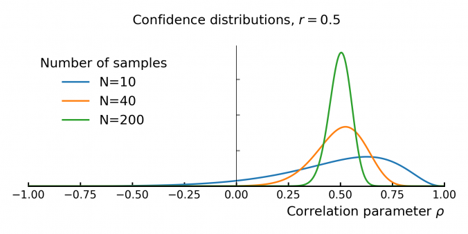
Correlation is everywhere in finance. It’s the backbone of portfolio optimization, risk management, and models like the CAPM. The idea is simple: mix assets that don’t move in sync, and you can reduce risk without sacrificing too much return. But there’s a problem—correlation is usually taken at face value, even though it’s often some form of an estimate based on historical data. …and that estimate comes with uncertainty!
This matters because small errors in correlation can throw off portfolio models. If you overestimate diversification, your portfolio might be riskier than expected. If you underestimate it, you could miss out on returns. In models like the CAPM, where correlation helps determine expected returns, bad estimates can lead to bad decisions.
Despite this, some asset managers don’t give much thought to how unstable correlation estimates can be. In this post, we’ll dig into the uncertainty behind empirical correlation, and how to quantify it.
Continue readingThis is a fun project me and my son did over the weekend.
I’ve always wondered what was going on in president Bush’s mind right after he was informed about the 9/11 attack.
Using a technique called Eulerian Video Magnification we were able to estimate his heart rate, and compare it right before- and after learning about the attack.
In this post we describe a nice algorithm for computing implied interest rates upper- and lower-bounds from European option quotes. These bounds tell you what the highest and lowest effective interest rates are that you can get by depositing or borrowing risk-free money through combinations of option trades. Knowing these bounds allows you to do two things:
1. Compare implied interest rate levels in the option markets with other interest rate markets. If they don’t align then you do a combination of option trades to capture the difference.
2. Check if the best borrowing rate is higher than the lowest deposit rate. If this is not the case, then this means there is a tradable arbitrage opportunity in the market: you can trader a combination of options that effectively boils down to borrowing money at a certain rate, and at the same time depositing that money at a higher rate.
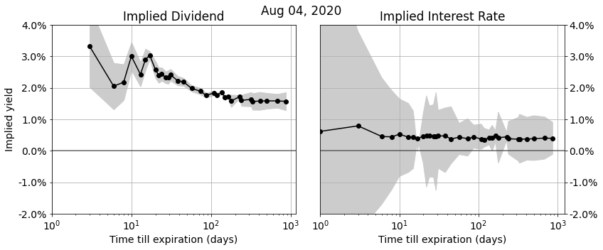
Continue readingIn this post we discuss the algorithms we use to accurately recover implied dividend and interest rates from option markets.
Implied dividends and interest rates show up in a wide variety of applications:
- to link future-, call-, and put-prices together in a consistent market view
- de-noise market (closing) prices of options and futures and stabilize PnL’s of option books
- give tighter true bid-ask spreads based on parity and arbitrage relationships
- compute accurate implied volatility smiles and surfaces
- provide predictive models and trading strategies with signals based on implied dividends, and implied interest rate information
Back-testing trading strategies is a dangerous business because there is a high risk you will keep tweaking your trading strategy model to make the back-test results better. When you do so, you’ll find out that after tweaking you have actually worsened the ‘live’ performance later on. The reason is that you’ve been overfitting your trading model to your back-test data through selection bias.
In this post we will use two techniques that help quantify and monitor the statistical significance of backtesting and tweaking:
- First, we analyze the performance of backtest results by comparing them against random trading strategies that similar trading characteristics (time period, number of trades, long/short ratio). This quantifies specifically how “special” the timing of the trading strategy is while keeping all other things equal (like the trends, volatility, return distribution, and patterns in the traded asset).
- Second, we analyse the impact and cost of tweaking strategies by comparing it against doing the same thing with random strategies. This allows us to see if improvements are significant, or simply what one would expect when picking the best strategy from a set of multiple variants.
The Python code snippet below uses the multiprocessing library to processes a list of tasks in parallel using a pool of 5 threads.
note: Python also has a multithreading library called “threading”, but it is well documented that Python multithreading doesn’t work for CPU-bound tasks due to Python’s Global Interpreter Lock (GIL), for more info google: “python multithreading gil”.
from multiprocessing import Process, Pool

import itertools
import time


def train(opt, delay=2.0):
    time.sleep(delay)
    return f'Done training {opt}'


# Grid search
grid = {
    'batch_size': [32, 64, 128],
    'learning_rate': [1E-4, 1E-3, 1E-2]
}


def main():
    settings_list = []
    for values in itertools.product(*grid.values()):
        settings_list.append( dict(zip(grid.keys(), values)) )

    with Pool(5) as p:
        print(p.map(train, settings_list))


if __name__ == "__main__":
    main()
Output
[
"Done training {'batch_size': 32, 'learning_rate': 0.0001}",
"Done training {'batch_size': 32, 'learning_rate': 0.001}",
"Done training {'batch_size': 32, 'learning_rate': 0.01}",
"Done training {'batch_size': 64, 'learning_rate': 0.0001}",
"Done training {'batch_size': 64, 'learning_rate': 0.001}",
"Done training {'batch_size': 64, 'learning_rate': 0.01}",
"Done training {'batch_size': 128, 'learning_rate': 0.0001}",
"Done training {'batch_size': 128, 'learning_rate': 0.001}",
"Done training {'batch_size': 128, 'learning_rate': 0.01}"
]
Python’s Itertools offers a great solution when you want to do a grid-search for optimal hyperparameter values, -or in general generate sets of experiments-.
In the code fragment below we generate experiment settings (key-value pairs stored in dictionaries) for all combinations of batch sizes and learning rates.
import itertools

# General settings
base_settings = {'epochs': 10}

# Grid search
grid = {
    'batch_size': [32, 64, 128],
    'learning_rate': [1E-4, 1E-3, 1E-2]
}

# Loop over al grid search combinations
for values in itertools.product(*grid.values()):
    point = dict(zip(grid.keys(), values))

    # merge the general settings
    settings = {**base_settings, **point}

    print(settings)
output:
{'epochs': 10, 'batch_size': 32, 'learning_rate': 0.0001}
{'epochs': 10, 'batch_size': 32, 'learning_rate': 0.001}
{'epochs': 10, 'batch_size': 32, 'learning_rate': 0.01}
{'epochs': 10, 'batch_size': 64, 'learning_rate': 0.0001}
{'epochs': 10, 'batch_size': 64, 'learning_rate': 0.001}
{'epochs': 10, 'batch_size': 64, 'learning_rate': 0.01}
{'epochs': 10, 'batch_size': 128, 'learning_rate': 0.0001}
{'epochs': 10, 'batch_size': 128, 'learning_rate': 0.001}
{'epochs': 10, 'batch_size': 128, 'learning_rate': 0.01}
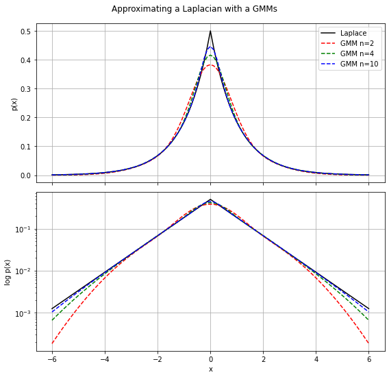
The Laplacian distribution is an interesting alternative building-block compared to the Gaussian distribution because it has much fatter tails. A drawback might be that some nice analytical properties that Gaussian distribution gives you don’t easily translate to Laplacian distributions. In those cases, it can be handy to approximate the Laplacian distribution with a mixture of Gaussians. The following approximation can then be uses
![]()
def laplacian_gmm(n=4):
    # all components have the same weight
    weights = np.repeat(1.0/n, n)

    # centers of the n bins in the interval [0,1]
    uniform = np.arange(0.5/n, 1.0, 1.0/n)

    # Uniform- to Exponential-distribution transform
    sigmas = np.array(-2*np.log(uniform))**.5
    return weights, sigmas

def laplacian_gmm_pdf(x, n=4):
    weights, sigmas = laplacian_gmm(n)
    p = np.zeros_like(x)
    for i in range(n):
        p += weights[i] * norm(loc=0, scale=sigmas[i]).pdf(x)
    return p
