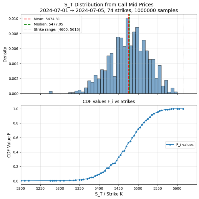
simulation – SITMO Machine Learning

For a single maturity, European call prices encode the risk-neutral distribution of the underlying. You can turn them into Monte Carlo samples without fitting a model or estimating a density.

For strikes $K_0 < … < K_n$ with call prices $C_0, …, C_n$ , define

$F_i = 1 + e^{rT} \frac{C_{i+1}-C_i}{K_{i+1}-K_i}, \quad F_0 = 0, \quad F_n = 1$

This is a discrete approximation of the cumulative distribution function of $S_T$ .

To sample:

Draw $U \sim Uniform(0,1)$
Find $i$ such that $F_i \le U < F_{i+1}$
Set

$S_T = K_i + (K_{i+1}-K_i)\frac{U-F_i}{F_{i+1}-F_i}$

Repeat for as many samples as needed.

This produces risk-neutral samples directly from observed call prices using only simple finite differences. It’s fully model-free, requires no volatility surface fitting, and preserves arbitrage constraints!

Below and example results from S&P500 option prices:

The Current Market Shake-Up

Last week, global stock markets faced a sharp and sudden correction. The S&P 500 dropped 10% in just two trading days, its worst weekly since the Covid crash 5 years ago.

Big drops like this remind us that market volatility isn’t random, it tends to stick around once it starts. When markets fall sharply, that volatility often continues for days or even weeks. And importantly, negative returns usually lead to bigger increases in volatility than positive returns do. This behavior is called asymmetry, and it’s something that simple models don’t handle very well.

In this post, we’ll explore the Glosten-Jagannathan-Runkle GARCH model (GJR-GARCH), a widely-used asymmetric volatility model. We’ll apply it to real S&P 500 data, simulate future price and volatility scenarios, and interpret what it tells us about market expectations.

Tag: simulation

Sampling Stock Prices Directly from Option Prices

Forecasting Current Market Turbulence with the GJR-GARCH Model

The Current Market Shake-Up