Tag: correlation

Using Fractional Brownian Motion in Finance: Simulation, Calibration, Prediction and Real World Examples

April 5, 2025 / Thijs van den Berg

Long Memory in Financial Time Series

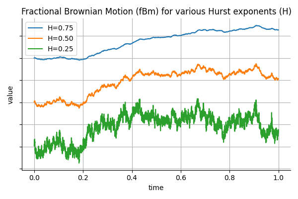
In finance, it is common to model asset prices and volatility using stochastic processes that assume independent increments, such as geometric Brownian motion. However, empirical observations suggest that many financial time series exhibit long memory or persistence. For example, volatility shocks can persist over extended periods, and high-frequency order flow often displays non-negligible autocorrelation. To capture such behavior, fractional Brownian motion (fBm) introduces a flexible framework where the memory of the process is governed by a single parameter: the Hurst exponent.

Building Correlation Matrices with Controlled Eigenvalues: A Simple Algorithm

March 15, 2025 / Thijs van den Berg

In some cases, we need to construct a correlation matrix with a predefined set of eigenvalues, which is not trivial since arbitrary symmetric matrices with a given set of eigenvalues may not satisfy correlation constraints (e.g., unit diagonal elements).

A practical method to generate such matrices is based on the Method of Alternating Projections (MAP), as introduced by Waller (2018). This approach iteratively adjusts a matrix between two sets until convergence. It goes like this:

Finding the Nearest Valid Correlation Matrix with Higham’s Algorithm

March 12, 2025 / Thijs van den Berg

Introduction

In quantitative finance, correlation matrices are essential for portfolio optimization, risk management, and asset allocation. However, real-world data often results in correlation matrices that are invalid due to various issues:

Merging Non-Overlapping Datasets: If correlations are estimated separately for different periods or asset subsets and then stitched together, the resulting matrix may lose its positive semidefiniteness.
Manual Adjustments: Risk/assert managers sometimes override statistical estimates based on qualitative insights, inadvertently making the matrix inconsistent.
Numerical Precision Issues: Finite sample sizes or noise in financial data can lead to small negative eigenvalues, making the matrix slightly non-positive semidefinite.

Fig 5. The impact of number of samples on the variance of the confidence distribution.

Understanding the Uncertainty of Correlation Estimates

March 9, 2025 / Thijs van den Berg

Correlation is everywhere in finance. It’s the backbone of portfolio optimization, risk management, and models like the CAPM. The idea is simple: mix assets that don’t move in sync, and you can reduce risk without sacrificing too much return. But there’s a problem—correlation is usually taken at face value, even though it’s often some form of an estimate based on historical data. …and that estimate comes with uncertainty!

This matters because small errors in correlation can throw off portfolio models. If you overestimate diversification, your portfolio might be riskier than expected. If you underestimate it, you could miss out on returns. In models like the CAPM, where correlation helps determine expected returns, bad estimates can lead to bad decisions.

Despite this, some asset managers don’t give much thought to how unstable correlation estimates can be. In this post, we’ll dig into the uncertainty behind empirical correlation, and how to quantify it.