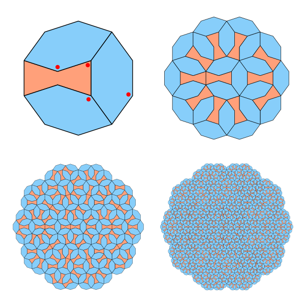
Tag: algorithm

Sampling Stock Prices Directly from Option Prices

February 2, 2026 / Thijs van den Berg

For a single maturity, European call prices encode the risk-neutral distribution of the underlying. You can turn them into Monte Carlo samples without fitting a model or estimating a density.

For strikes $K_0 < … < K_n$ with call prices $C_0, …, C_n$ , define

$F_i = 1 + e^{rT} \frac{C_{i+1}-C_i}{K_{i+1}-K_i}, \quad F_0 = 0, \quad F_n = 1$

This is a discrete approximation of the cumulative distribution function of $S_T$ .

To sample:

Draw $U \sim Uniform(0,1)$
Find $i$ such that $F_i \le U < F_{i+1}$
Set

$S_T = K_i + (K_{i+1}-K_i)\frac{U-F_i}{F_{i+1}-F_i}$

Repeat for as many samples as needed.

This produces risk-neutral samples directly from observed call prices using only simple finite differences. It’s fully model-free, requires no volatility surface fitting, and preserves arbitrage constraints!

Below and example results from S&P500 option prices:

A Tiling That Never Repeats

April 11, 2025 / Thijs van den Berg

This image below shows a tiling made from just two simple shapes, arranged in a pattern that never repeats. You can extend it as far as you like, and it will keep growing in complexity without ever falling into a regular cycle. That property alone makes it interesting, but the background is even better.

A Curve That Fills Space

April 10, 2025 / Thijs van den Berg

Here’s a short snippet that draws the Hilbert space-filling curve using a recursive approach.

It sounds counterintuitive. A curve normally has no area, it’s just a line. But a space-filling curve is a special type of curve that gets arbitrarily close to every point in a 2D square. If you keep refining it, the curve passes so densely through the space that it effectively covers the entire square. In the mathematical limit, it touches every point.

Building Correlation Matrices with Controlled Eigenvalues: A Simple Algorithm

March 15, 2025 / Thijs van den Berg

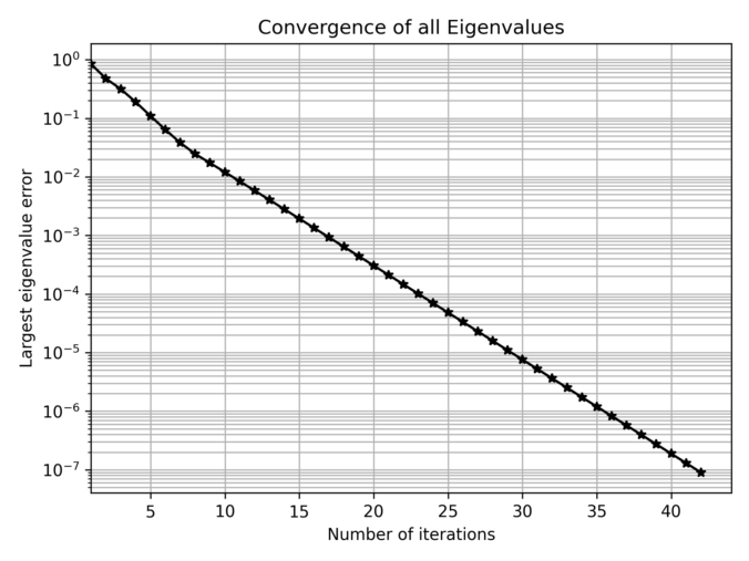
In some cases, we need to construct a correlation matrix with a predefined set of eigenvalues, which is not trivial since arbitrary symmetric matrices with a given set of eigenvalues may not satisfy correlation constraints (e.g., unit diagonal elements).

A practical method to generate such matrices is based on the Method of Alternating Projections (MAP), as introduced by Waller (2018). This approach iteratively adjusts a matrix between two sets until convergence. It goes like this:

Finding the Nearest Valid Correlation Matrix with Higham’s Algorithm

March 12, 2025 / Thijs van den Berg

Introduction

In quantitative finance, correlation matrices are essential for portfolio optimization, risk management, and asset allocation. However, real-world data often results in correlation matrices that are invalid due to various issues:

Merging Non-Overlapping Datasets: If correlations are estimated separately for different periods or asset subsets and then stitched together, the resulting matrix may lose its positive semidefiniteness.
Manual Adjustments: Risk/assert managers sometimes override statistical estimates based on qualitative insights, inadvertently making the matrix inconsistent.
Numerical Precision Issues: Finite sample sizes or noise in financial data can lead to small negative eigenvalues, making the matrix slightly non-positive semidefinite.

Efficient Rolling Median with the Two-Heaps Algorithm. O(log n)

March 10, 2025 / Thijs van den Berg

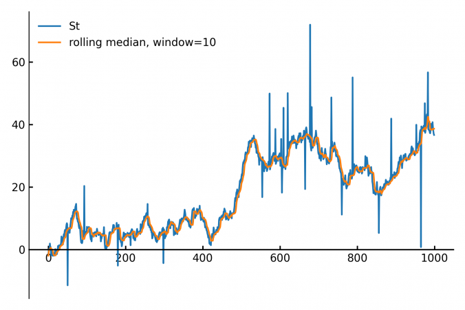
Calculating the median of data points within a moving window is a common task in fields like finance, real-time analytics and signal processing. The main applications are anomal- and outlier-detection / removal.