When building trading strategies, a crucial decision is how to translate market information into trading actions.
Traditional supervised learning approaches tackle this by predicting price movements directly, essentially guessing if the price will move up or down.
Typically, we decide on labels in supervised learning by asking something like: “Will the price rise next week?” or “Will it increase more than 2% over the next few days?” While these are intuitive choices, they often seem arbitrarily tweaked and overlook the real implications on trading strategies. Choices like these silently influence trading frequency, transaction costs, risk exposure, and strategy performance, without clearly tying these outcomes to specific label modeling decisions. There’s a gap here between the supervised learning stage (forecasting) and the actual trading decisions, which resemble reinforcement learning actions.
In this post, I present a straightforward yet rigorous solution that bridges this gap, by formulating label selection itself as an optimization problem. Instead of guessing or relying on intuition, labels are derived from explicitly optimizing a defined trading performance objective -like returns or Sharpe ratio- while respecting realistic constraints such as transaction costs or position limits. The result is labeling that is no longer arbitrary, but transparently optimal and directly tied to trading performance.
Continue reading
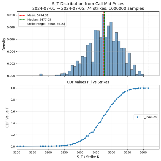
 with call prices
  , define
![\[F_i = 1 + e^{rT} \frac{C_{i+1}-C_i}{K_{i+1}-K_i}, \quad F_0 = 0, \quad F_n = 1\]](https://www.sitmo.com/wp-content/ql-cache/quicklatex.com-67e0ef1fe3b0d34ac0811466d99b4ec6_l3.png "Rendered by QuickLaTeX.com")
 .
.
 such that
![\[S_T = K_i + (K_{i+1}-K_i)\frac{U-F_i}{F_{i+1}-F_i}\]](https://www.sitmo.com/wp-content/ql-cache/quicklatex.com-c33ca9b41ab9bb22d5436e82a1f3ef9e_l3.png "Rendered by QuickLaTeX.com")