
Gravitational lensing is one of the most beautiful predictions of general relativity.
When a massive object, like a galaxy or black hole, lies between a distant light source and an observer, the gravitational field bends the path of light rays, distorting and duplicating the image of the background object. In this post, we’ll build a simple but realistic raytracer that simulates this phenomenon in two dimensions.
Author: Thijs van den Berg (Page 2 of 3)
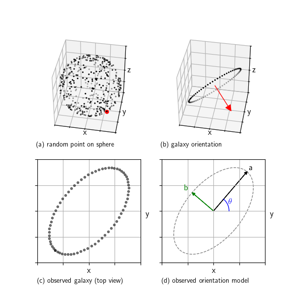
When we look at galaxies through a telescope, we see them as ellipses. But real galaxies are 3D disks randomly oriented in space. This post shows how we can simulate that: we start with a random orientation, project a flat disk into the 2D image plane, and extract the observed ellipse parameters. This setup helps us understand what shape distributions we expect to see in the absence of structures like gravitational lensing and clustering.
In research we can analyse and compare the properties of this pure random reference model against real observations to look for subtle distortions
Continue reading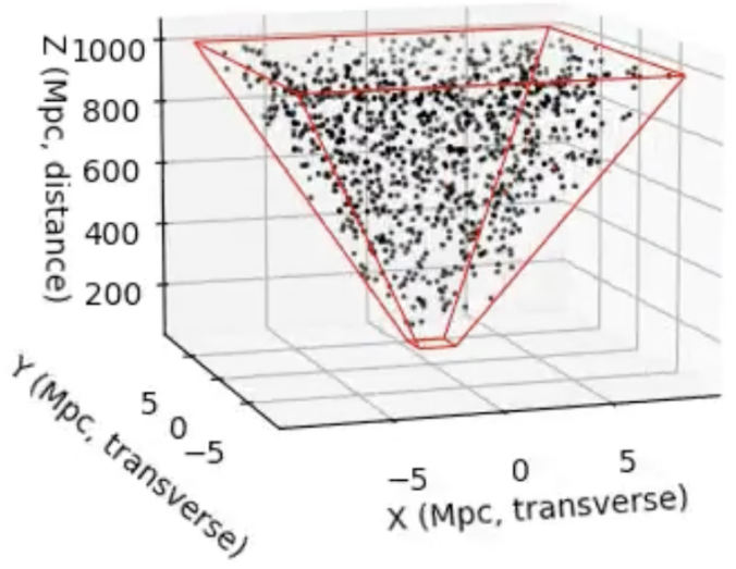
When we look at an astronomical image, we see a 2D projection of a 3D universe. But suppose we want to simulate the distribution of galaxies behind that image, for example, to generate synthetic data, test detection algorithms, or check if real galaxy distributions statistically deviate from what we’d expect under uniformity. To do this, we need a way to sample galaxies uniformly in 3D space, restricted to the cone of space visible in an image.
Continue reading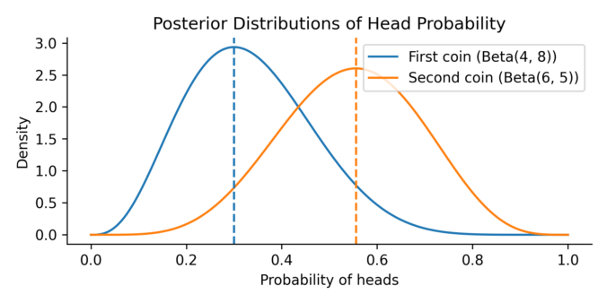
Imagine you’re comparing two trading strategies. One has made a handful of successful trades over the past month, while the other shows a different success pattern over a slightly shorter period. Both show promise, but which one truly performs better? And more importantly, how confident can we be in that judgment, given such limited data?
To explore this, let’s turn to a simpler but mathematically equivalent situation: comparing two coins. The first coin is flipped 10 times and lands heads 3 times. The second coin is flipped 9 times and lands heads 5 times. We want to know: what is the probability that the second coin has a higher chance of landing heads than the first?
Continue reading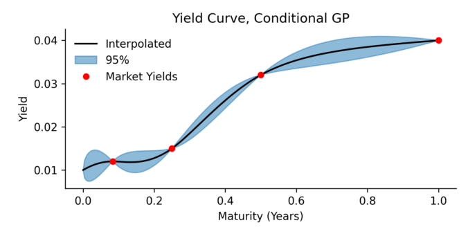
Here we present a yield curve interpolation method, one that’s based on conditioning a stochastic model on a set of market yields. The concept is closely related to a Brownian bridge where you generate scenario according to an SDE, but with the extra condition that the start and end of the scenario’s must have certain values. In this paper we use Gaussian process regression to generalization the Brownian bridge and allows for more complicated conditions. As an example, we condition the Vasicek spot interest rate model on a set of yield constraints and provide an analytical solution.
The resulting model can be applied in several areas:
- Monte Carlo scenario generation
- Yield curve interpolation
- Estimating optimal hedges, and the associated risk for non tradable products
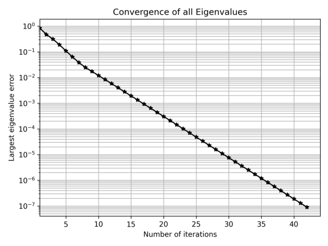
In some cases, we need to construct a correlation matrix with a predefined set of eigenvalues, which is not trivial since arbitrary symmetric matrices with a given set of eigenvalues may not satisfy correlation constraints (e.g., unit diagonal elements).
A practical method to generate such matrices is based on the Method of Alternating Projections (MAP), as introduced by Waller (2018). This approach iteratively adjusts a matrix between two sets until convergence. It goes like this:
Continue reading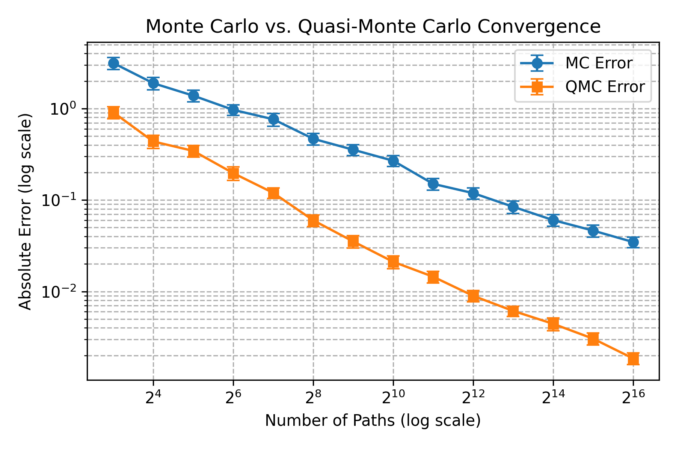
In this post, we discuss the usefulness of low-discrepancy sequences (LDS) in finance, particularly for option pricing. Unlike purely random sampling, LDS methods generate points that are more evenly distributed over the sample space. This uniformity reduces the gaps and clustering seen in standard Monte Carlo (MC) sampling and improves convergence in numerical integration problems.
A key measure of sampling quality is discrepancy, which quantifies how evenly a set of points covers the space. Low-discrepancy sequences minimize this discrepancy, leading to faster convergence in high-dimensional simulations.
Continue reading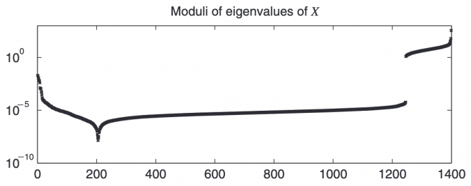
Introduction
In quantitative finance, correlation matrices are essential for portfolio optimization, risk management, and asset allocation. However, real-world data often results in correlation matrices that are invalid due to various issues:
- Merging Non-Overlapping Datasets: If correlations are estimated separately for different periods or asset subsets and then stitched together, the resulting matrix may lose its positive semidefiniteness.
- Manual Adjustments: Risk/assert managers sometimes override statistical estimates based on qualitative insights, inadvertently making the matrix inconsistent.
- Numerical Precision Issues: Finite sample sizes or noise in financial data can lead to small negative eigenvalues, making the matrix slightly non-positive semidefinite.
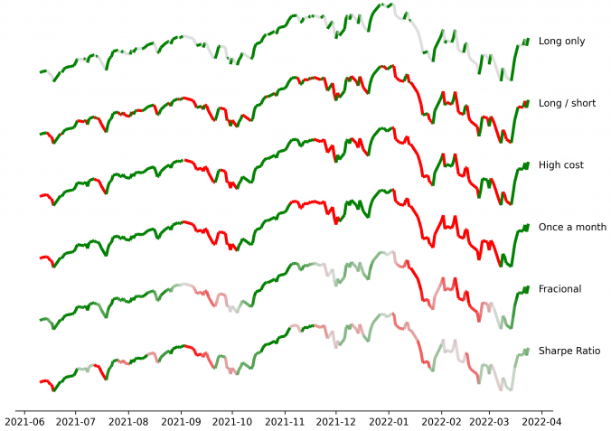
When building trading strategies, a crucial decision is how to translate market information into trading actions.
Traditional supervised learning approaches tackle this by predicting price movements directly, essentially guessing if the price will move up or down.
Typically, we decide on labels in supervised learning by asking something like: “Will the price rise next week?” or “Will it increase more than 2% over the next few days?” While these are intuitive choices, they often seem arbitrarily tweaked and overlook the real implications on trading strategies. Choices like these silently influence trading frequency, transaction costs, risk exposure, and strategy performance, without clearly tying these outcomes to specific label modeling decisions. There’s a gap here between the supervised learning stage (forecasting) and the actual trading decisions, which resemble reinforcement learning actions.
In this post, I present a straightforward yet rigorous solution that bridges this gap, by formulating label selection itself as an optimization problem. Instead of guessing or relying on intuition, labels are derived from explicitly optimizing a defined trading performance objective -like returns or Sharpe ratio- while respecting realistic constraints such as transaction costs or position limits. The result is labeling that is no longer arbitrary, but transparently optimal and directly tied to trading performance.
Continue reading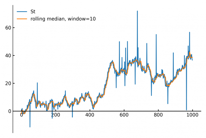
Calculating the median of data points within a moving window is a common task in fields like finance, real-time analytics and signal processing. The main applications are anomal- and outlier-detection / removal.
Continue reading