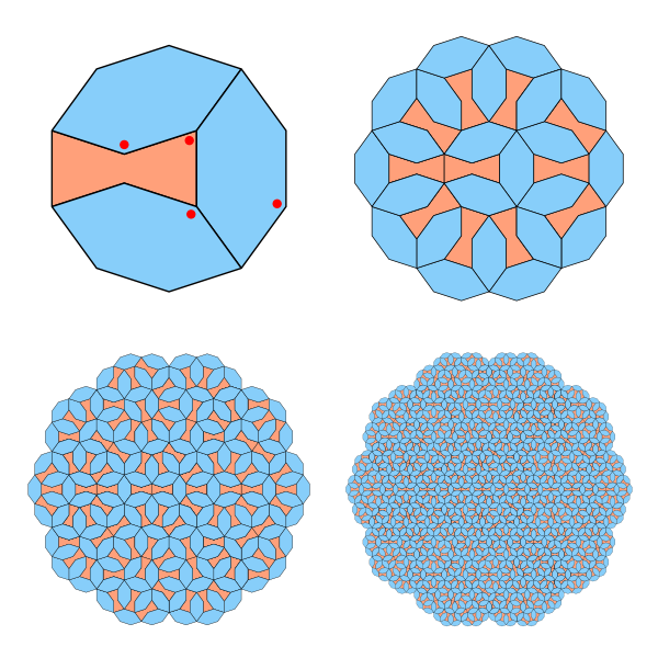
This image below shows a tiling made from just two simple shapes, arranged in a pattern that never repeats. You can extend it as far as you like, and it will keep growing in complexity without ever falling into a regular cycle. That property alone makes it interesting, but the background is even better.
Continue reading
Here’s a short snippet that draws the Hilbert space-filling curve using a recursive approach.
It sounds counterintuitive. A curve normally has no area, it’s just a line. But a space-filling curve is a special type of curve that gets arbitrarily close to every point in a 2D square. If you keep refining it, the curve passes so densely through the space that it effectively covers the entire square. In the mathematical limit, it touches every point.
Continue reading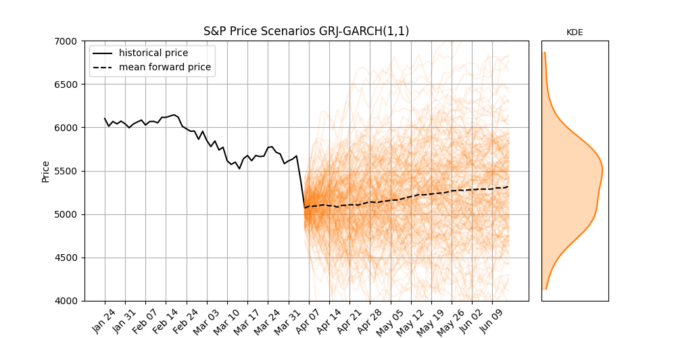
The Current Market Shake-Up
Last week, global stock markets faced a sharp and sudden correction. The S&P 500 dropped 10% in just two trading days, its worst weekly since the Covid crash 5 years ago.
Big drops like this remind us that market volatility isn’t random, it tends to stick around once it starts. When markets fall sharply, that volatility often continues for days or even weeks. And importantly, negative returns usually lead to bigger increases in volatility than positive returns do. This behavior is called asymmetry, and it’s something that simple models don’t handle very well.
In this post, we’ll explore the Glosten-Jagannathan-Runkle GARCH model (GJR-GARCH), a widely-used asymmetric volatility model. We’ll apply it to real S&P 500 data, simulate future price and volatility scenarios, and interpret what it tells us about market expectations.
Continue reading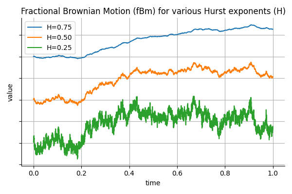
Long Memory in Financial Time Series
In finance, it is common to model asset prices and volatility using stochastic processes that assume independent increments, such as geometric Brownian motion. However, empirical observations suggest that many financial time series exhibit long memory or persistence. For example, volatility shocks can persist over extended periods, and high-frequency order flow often displays non-negligible autocorrelation. To capture such behavior, fractional Brownian motion (fBm) introduces a flexible framework where the memory of the process is governed by a single parameter: the Hurst exponent.
Continue reading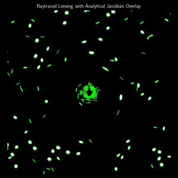
In the previous post, we built a simple gravitational lens raytracer that simulates how an image would be distorted when seen through a point-mass gravitational lens. That approach was fully numerical: we traced rays from each pixel and observed how they bent. But if we’re working with small, elliptical galaxies and want to understand how their shapes change statistically, we can use an analytical model based on the lensing Jacobian.
Continue reading
Gravitational lensing is one of the most beautiful predictions of general relativity.
When a massive object, like a galaxy or black hole, lies between a distant light source and an observer, the gravitational field bends the path of light rays, distorting and duplicating the image of the background object. In this post, we’ll build a simple but realistic raytracer that simulates this phenomenon in two dimensions.
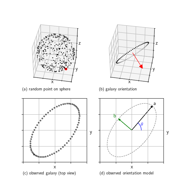
When we look at galaxies through a telescope, we see them as ellipses. But real galaxies are 3D disks randomly oriented in space. This post shows how we can simulate that: we start with a random orientation, project a flat disk into the 2D image plane, and extract the observed ellipse parameters. This setup helps us understand what shape distributions we expect to see in the absence of structures like gravitational lensing and clustering.
In research we can analyse and compare the properties of this pure random reference model against real observations to look for subtle distortions
Continue reading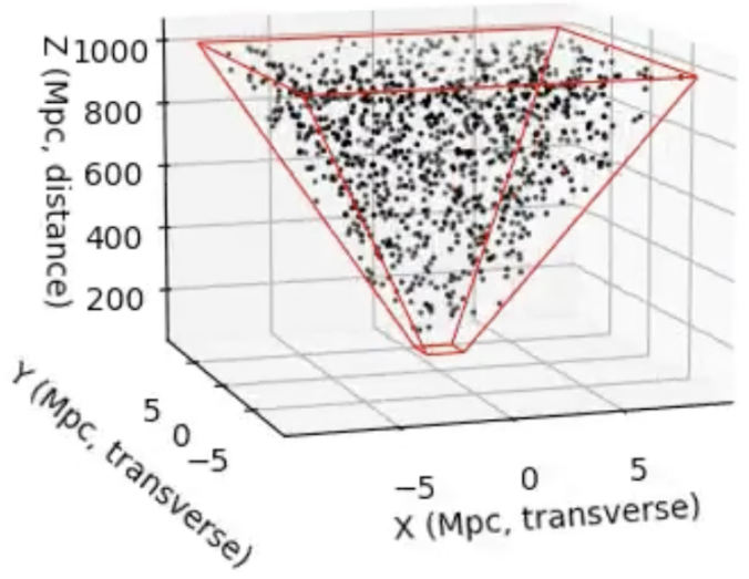
When we look at an astronomical image, we see a 2D projection of a 3D universe. But suppose we want to simulate the distribution of galaxies behind that image, for example, to generate synthetic data, test detection algorithms, or check if real galaxy distributions statistically deviate from what we’d expect under uniformity. To do this, we need a way to sample galaxies uniformly in 3D space, restricted to the cone of space visible in an image.
Continue reading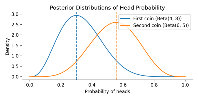
Imagine you’re comparing two trading strategies. One has made a handful of successful trades over the past month, while the other shows a different success pattern over a slightly shorter period. Both show promise, but which one truly performs better? And more importantly, how confident can we be in that judgment, given such limited data?
To explore this, let’s turn to a simpler but mathematically equivalent situation: comparing two coins. The first coin is flipped 10 times and lands heads 3 times. The second coin is flipped 9 times and lands heads 5 times. We want to know: what is the probability that the second coin has a higher chance of landing heads than the first?
Continue reading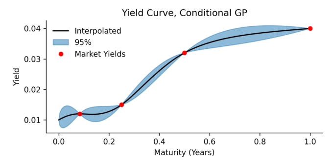
Here we present a yield curve interpolation method, one that’s based on conditioning a stochastic model on a set of market yields. The concept is closely related to a Brownian bridge where you generate scenario according to an SDE, but with the extra condition that the start and end of the scenario’s must have certain values. In this paper we use Gaussian process regression to generalization the Brownian bridge and allows for more complicated conditions. As an example, we condition the Vasicek spot interest rate model on a set of yield constraints and provide an analytical solution.
The resulting model can be applied in several areas:
- Monte Carlo scenario generation
- Yield curve interpolation
- Estimating optimal hedges, and the associated risk for non tradable products