Another Post – SITMO Machine Learning

Denoising Correlation Matrices for More Stable Portfolio Optimization

November 7, 2025 / Thijs van den Berg

Introduction

Portfolio optimization lies at the heart of asset management, guiding investment strategies from risk minimization to return maximization. Many of the most widely used allocation methods such as minimum variance, maximum Sharpe ratio, and risk parity rely on the inverse of the correlation matrix to compute optimal portfolio weights. However, if the correlation matrix is poorly conditioned (i.e., has a high condition number, which we will go into below), its inverse becomes highly sensitive to small changes in correlation estimates, leading to unstable portfolio allocations.

The problem arises because empirical correlation matrices, estimated from historical data, contain both true underlying structure and random sample noise. This noise can distort the eigenspectrum, leading to small eigenvalues that make inversion unstable. To mitigate this, we apply denoising techniques based on Random Matrix Theory (RMT) to improve stability. The goal is to reduce sensitivity in the inverse correlation matrix, making portfolio allocations more robust to estimation noise.

Correlation Matrix Inversion in Portfolio Optimization

The following table illustrates how the inverse correlation (or covariance) matrix appears in common asset allocation methods:

\[w^* = \frac{\Sigma^{-1} \mathbf{1}}{\mathbf{1}^T \Sigma^{-1} \mathbf{1}}\]

Optimization Objective	Portfolio Weights Formula
Minimum-Variance Portfolio	$w^* = \frac{\Sigma^{-1} \mathbf{1}}{\mathbf{1}^T \Sigma^{-1} \mathbf{1}}$
Mean-Variance (Markowitz)	$w^* = \lambda \Sigma^{-1} \mu$
Maximum Sharpe Ratio	$w^* = \frac{\Sigma^{-1} (\mu - r_f \mathbf{1})}{\mathbf{1}^T \Sigma^{-1} (\mu - r_f \mathbf{1})}$
Risk Parity	solve $w_i (\Sigma w)_i = \frac{1}{N} \sum_j w_j (\Sigma w)_j$
Maximum Diversification	$w^* = \frac{\Sigma^{-1} \sigma}{\mathbf{1}^T \Sigma^{-1} \sigma}$

A correlation matrix can be viewed as a linear transformation that stretches or compresses a set of uncorrelated points into a correlated structure. The eigenvectors of the correlation matrix define the axes and the directions of this transformation, while the eigenvalues determine how much scaling occurs along each axis.

Visualizing Correlation and Its Inverse

Below, we illustrate this concept with three side-by-side scatter plots:

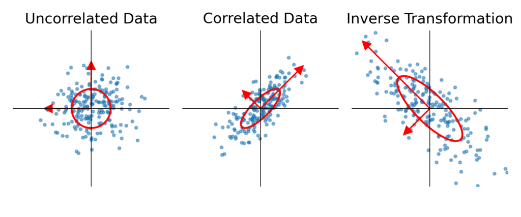
Fig 1. Correlations and their relation to portfolio weights

Left: Uncorrelated data (standard normal distribution, spherical shape).
Middle: Data transformed by a correlation matrix (stretched into an elliptical shape).
Right: The effect of inverting the correlation matrix, illustrating how portfolio optimization weights are influenced.

The inverse transformation undoes this stretching/squashing process. If a correlation matrix has very small eigenvalues, these correspond to directions that are nearly collapsed, meaning their inverse will explode, leading to extreme allocations in the optimization process.

How Do the Vectors in the Inverse Transform Relate to Portfolio Weights?

The vectors plotted in the inverse transformation panel correspond to the principal directions of risk in the correlation matrix. These are the eigenvectors, and their associated eigenvalues determine how much the matrix stretches or contracts data in each direction.

Portfolio weights are most sensitive to:

Small eigenvalues in $\Sigma$ , which become large when inverted.
Uncertainty in the direction of the eigenvectors, which determines how weight is distributed across assets.

If a correlation matrix has one very small eigenvalue, its inverse explodes, meaning any small change in correlation structure leads to a huge shift in portfolio weights. This is why a poorly conditioned correlation matrix leads to unstable allocations.

Uncertaintly in Correlation Estimates

In theory, we assume that the correlation matrix reflects true relationships between assets, but in practice, correlations are estimated from finite historical data and are subject to sample noise. Each correlation estimate is just an approximation of the true underlying structure, and these estimates fluctuate depending on the dataset used. The problem is twofold:

estimated historical correlations are notoriously imprecise, the values you estimate are very noisy
small variations in estimated correlations can -under certain conditions- significantly distort the portfolio weights, this happend when we have small eigenvalues and when the condition number is high

This issue becomes even more pronounced in large correlation matrices in a multi-asset setting, the more assets included, the higher the probability of encountering highly correlated noise events that introduce small eigenvalues. These spurious correlations arise purely due to randomness, yet they can significantly impact portfolio optimization by creating unstable inverse matrices.

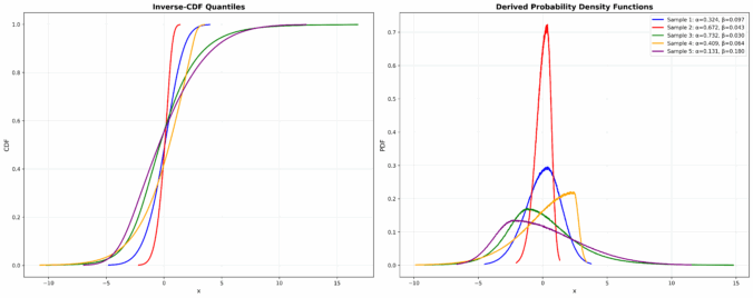
In fig 2., in the left column -top to bottom-, we generated 3 samples of random data that was generated using the same true correlation of 0.8, yet the estimated correlation differs across samples, varying from 0.52 to 0.92. The key takeaway is that even when the true correlation structure is fixed, its empirical estimate varies due to sampling noise. This is a fundamental challenge in finance, where limited data availability makes robust correlation estimation difficult.

Fig 2. Sample noise and its impact on portfolio weights

The right column shows the effect of inverting the noisy empirical correlation matrix. The inverse correlation matrix is highly unstable across different samples. This instability is caused by:

Uncertainty in the estimated correlation matrix
- Since correlation estimates fluctuate due to sample noise, their eigenvectors also shift unpredictably, affecting the inverse.
High correlation leading to small eigenvalues
- When assets are highly correlated, the correlation matrix has small eigenvalues, making inversion problematic.
- Small eigenvalues become large when inverted, leading to exploding elements in the inverse correlation matrix, which in turn makes portfolio optimization highly sensitive to small changes in correlation estimates.

This is why raw empirical correlation matrices often produce unstable portfolio allocations. Without regularization or denoising, small changes in historical data lead to drastically different asset weights, making any optimization unreliable.

Random Matrix Theory and the Marčenko-Pastur Distribution

When the number of assets is large compared to the number of observations, the empirical correlation matrix contains a significant amount of noise. The question then becomes: how do we distinguish true correlations from random noise?

This is where Random Matrix Theory (RMT) provides valuable insights. RMT studies the statistical properties of large random matrices. One of its key results is the Marčenko-Pastur distribution, which describes the expected distribution of eigenvalues when a correlation matrix is purely random -i.e., when the observed correlations contain no meaningful structure-.

The Marčenko-Pastur distribution describes the density of eigenvalues for a random covariance matrix constructed from independent Gaussian variables. The density function is given by:

$p(\lambda) = \frac{\sqrt{(\lambda_{+} - \lambda)(\lambda - \lambda_{-})}}{2\pi \sigma^2 q \lambda}$

where:

$\lambda$ represents the eigenvalues,
$\sigma^2$ is the true variance of the underlying data,
$q = \frac{T}{N}$ is the aspect ratio (i.e., the number of time periods $T$ divided by the number of assets $N$ ),
$\lambda_{-}$ and $\lambda_{+}$ are the theoretical lower and upper bounds of the eigenvalue spectrum, given by:

$\lambda_{\pm} = \sigma^2 (1 \pm \sqrt{q})^2$

This distribution serves as a benchmark for identifying noise in empirical correlation matrices: any eigenvalues inside the Marčenko-Pastur range are likely due to randomness, while eigenvalues outside this range may represent genuine structure.

To build intuition, we plot the Marčenko-Pastur distribution for different values of the aspect rati0 $q=\frac{T}{N}$ . This helps us see how the shape of the eigenvalue spectrum changes as we adjust the amount of data used to estimate correlations, or adjust the number of assets.

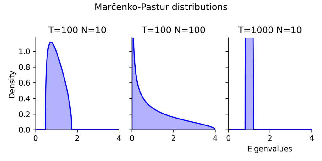
The three panels in (Fig 3) illustrate how the distribution of eigenvalues changes depending on the number of assets (N) and historical observations (T). The practical takeaway is clear: the ratio of historical data to assets strongly influences the stability of portfolio weights.

Left Panel: A somewhat typical case (T=100, N=10)

This represents a somewhat typical real-world scenario where we have more historical data than assets, but not by an overwhelming margin.

The Marčenko-Pastur distribution tells us that any eigenvalue below ~1.8 is likely just noise.
This means that many of the factors that appear significant in the correlation matrix are actually random fluctuations.
The inverse correlation matrix will still be somewhat stable, but there is a risk of unstable portfolio allocations if the condition number is high.

Middle Panel: A Bad Situation (T=100, N=100)

This is a worst-case scenario where the number of historical observations matches the number of assets.

The entire eigenvalue spectrum is stretched, meaning that even factors up to an eigenvalue of 4 are likely noise.
The smallest eigenvalue is likely close to zero, meaning that inverting the correlation matrix will be extremely unstable.
Portfolio optimizations in this setting will produce highly erratic weights that change drastically with small fluctuations in data.

This is a problem in high-dimensional finance, where investors want to include a large number of assets fro large universes but only have limited historical data. Without regularization, such matrices produce portfolio weights that are effectively meaningless.

Right Panel: A Well-Conditioned Case (T=1000, N=10)

This is the ideal scenario, where we have 100× more data than assets.

The smallest eigenvalue due to noise is still likely around 1, meaning that all eigenvalues are well-separated from zero.
This ensures that the correlation matrix inversion is stable, and portfolio weights remain robust.
Even if correlations change slightly, the impact on portfolio allocations is minimal.

Denoising the Correlation Matrix to Stabilize Portfolio Weights

We’ve seen how sample noise in correlation estimates leads to small eigenvalues, which in turn cause instability when inverting the correlation matrix. Now, we introduce a denoising strategy that helps reduce this instability, making portfolio allocations more robust.

The key idea is simple: we need to separate true structure (signal) from random fluctuations (noise) and then modify the noise-dominated parts of the correlation matrix to improve its condition number.

Step 1: Estimating the Amount of Noise in the Correlation Matrix

The eigenvalues of a correlation matrix represent the variance explained by different factors. For an $N \times N$ correlation matrix, the sum of its eigenvalues is always equal to $N$ :

$\sum_{i=1}^{N} \lambda_i = N$

This means that if there is real structure in the correlations, the signal-related eigenvalues will be larger, while the noise-related eigenvalues must be smaller to keep the sum constant.

To determine how much of the matrix is noise, we estimate the amount of variance explained by noise eigenvalues using maximum likelihood estimation (MLE). The idea is to fit the Marčenko-Pastur distribution to the empirical eigenvalues and estimate the variance of the random noise component. Any eigenvalue that is small enough to be explained by random noise is considered not meaningful.

At this stage, we have:

A separation between “signal” and “noise” eigenvalues.
An estimate of the noise level, which tells us how much distortion exists.

Step 2: Modifying the Smallest Eigenvalues to Reduce Instability

Once we identify the noise-dominated eigenvalues, the next step is modifying them to reduce their impact on portfolio weights.

Since the sum of eigenvalues must remain $N$ , simply increasing the smallest ones would require decreasing others, potentially distorting the true structure. Instead, a more stable approach is to replace all the noise-related eigenvalues with their average:

$\lambda_{\text{new}} = \frac{1}{K} \sum_{i \in \text{noise}} \lambda_i$

where $K$ is the number of noisy eigenvalues.

This modification has several key benefits:

It maximizes the smallest eigenvalue, improving the condition number.
It maintains the total sum of eigenvalues, preserving the overall structure of the correlation matrix.
It leaves the signal eigenvectors untouched, ensuring that meaningful correlations remain intact.

By applying this transformation, we stabilize the inverse correlation matrix, leading to portfolio weights that are far less sensitive to small changes in correlation estimates.

Releasing the GARCH Densities Dataset: 1,000 Trillion Simulations for Financial AI

October 16, 2025 / Thijs van den Berg

huggingface.co/datasets/sitmo/garch_densities

We’ve released a new open dataset on Hugging Face: GARCH Densities, a large-scale benchmark for density estimation, option pricing, and risk modeling in quantitative finance.

Created with Paul Wilmott, this dataset contains simulations from the GJR-GARCH model with Hansen skewed-t innovations. Each row links a parameter set

$\Theta = (\alpha, \gamma, \beta, \text{var0}, \eta, \lambda)$

to the inverse-CDF quantiles of terminal returns over multiple maturities.

Dataset highlights:

~1,000 trillion simulated price paths across 6D parameter space
Quantiles of normalized returns at 512 probability levels
Low-discrepancy Sobol sampling under $\alpha+\gamma+\beta < 0.95$
zstd-compressed Parquet shards (~145 MB each, streaming-friendly)
CC-BY-4.0 licensed — free for academic and commercial use

Applications:

Learning $\Theta \mapsto$ return distributions (pretrained pricing models)
Fast neural surrogates for Monte Carlo simulation
Option pricing, VaR/CVaR, and volatility surface modeling
Benchmarking generative and density estimation models

Example usage:

from datasets import load_dataset

ds = load_dataset("sitmo/garch_densities")
train, test = ds["train"], ds["test"]

print(train)
print(train.features)

PyTorch integration:

import torch
from torch.utils.data import DataLoader

param_cols = ["alpha","gamma","beta","var0","eta","lam","ti"]
train = train.with_format("torch", columns=param_cols + ["x"])
loader = DataLoader(train, batch_size=256, shuffle=True)

batch = next(iter(loader))
params, targets = torch.stack([batch[c] for c in param_cols], 1), batch["x"]
print(params.shape, targets.shape)

Goal: accelerate research on pretrained neural pricing models and scientific foundation models in finance — replacing slow Monte Carlo with fast, learned surrogates.

We’d love to see how researchers use this dataset. If you find it useful, consider sharing it or referencing it in your work.

License: CC-BY-4.0
Authors: Thijs van den Berg & Paul Wilmott
Link: https://huggingface.co/datasets/sitmo/garch_densities

New release of CGMM v0.4

October 16, 2025 / Thijs van den Berg

pip install cgmm

We’ve just released v0.4 of cgmm, our open-source library for Conditional Gaussian Mixture Modelling.

If you’re new to cgmm: it’s a flexible, data-driven way to model conditional distributions beyond Gaussian or linear assumptions. It can:

Model non-Gaussian distributions
Capture non-linear dependencies
Work in a fully data-driven way

This makes it useful in research and applied settings where complexity is the norm rather than the exception.

What’s new in this release:

Mixture of Experts (MoE): Softmax-gated experts with linear mean functions (Jordan & Jacobs, Hierarchical Mixtures of Experts and the EM Algorithm, Neural Computation, 1994)
Direct conditional likelihood optimization: EM algorithm implementation from Jaakkola & Haussler (Expectation-Maximization Algorithms for Conditional Likelihoods, ICML 2000)

New examples and applications include:

VIX volatility Monte Carlo simulation (non-linear, non-Gaussian SDEs)
Hourly and seasonal forecasts of temperature, windspeed, and light intensity
The IRIS dataset and other sklearn benchmarks
Generative modelling of MNIST handwritten digits

Explore more:

If you find this useful, please share it, give it a ⭐ on GitHub, or help spread the word. Your feedback and contributions make a big difference.

Not investment advice, the library continues to evolve, and we welcome ideas, feature requests, and real-world examples!

New open-source library: Conditional Gaussian Mixture Models (CGMM)

August 31, 2025 / Thijs van den Berg

pip install cgmm

I’ve released a small, lightweight Python library that learns conditional distributions and turns them e.g. into scenarios, fan charts, and risk bands with just a few lines of code. It’s built on top of scikit-learn (fits naturally into sklearn-style workflows and tooling).

Example usage:

In the figure below, a non-parametric model is fit on ΔVIX conditioned on the VIX level, so it naturally handles:

Non-Gaussian changes (fat tails / asymmetry), and
Non-linear, level-dependent drift (behavior differs when VIX is low vs. high).

Features:

Conditional densities and scenario generation for time series and tabular problems
Quantiles, prediction intervals, and median/mean paths vuia MC simulation
Multiple conditioning features (macro, technicals, regimes, etc.)
Lightweight & sklearn-friendly; open-source and free to use (BSD-3)

VIX example notebook: https://cgmm.readthedocs.io/en/latest/examples/vix_predictor.html

Call for examples & contributions:

Do you have a use-case we should showcase (rates, spreads, realized vol, token flows, energy, demand, order-book features…)?
Send a brief description or PR—examples will be attributed.
Contributions, issues, and feature requests are very welcome. And if you find this useful, please share or star the repo to help others discover it.

Not investment advice. The library is still work in progress!

A Tiling That Never Repeats

April 11, 2025 / Thijs van den Berg

This image below shows a tiling made from just two simple shapes, arranged in a pattern that never repeats. You can extend it as far as you like, and it will keep growing in complexity without ever falling into a regular cycle. That property alone makes it interesting, but the background is even better.

A Curve That Fills Space

April 10, 2025 / Thijs van den Berg

Here’s a short snippet that draws the Hilbert space-filling curve using a recursive approach.

It sounds counterintuitive. A curve normally has no area, it’s just a line. But a space-filling curve is a special type of curve that gets arbitrarily close to every point in a 2D square. If you keep refining it, the curve passes so densely through the space that it effectively covers the entire square. In the mathematical limit, it touches every point.

Forecasting Current Market Turbulence with the GJR-GARCH Model

April 6, 2025 / Thijs van den Berg

The Current Market Shake-Up

Last week, global stock markets faced a sharp and sudden correction. The S&P 500 dropped 10% in just two trading days, its worst weekly since the Covid crash 5 years ago.

Big drops like this remind us that market volatility isn’t random, it tends to stick around once it starts. When markets fall sharply, that volatility often continues for days or even weeks. And importantly, negative returns usually lead to bigger increases in volatility than positive returns do. This behavior is called asymmetry, and it’s something that simple models don’t handle very well.

In this post, we’ll explore the Glosten-Jagannathan-Runkle GARCH model (GJR-GARCH), a widely-used asymmetric volatility model. We’ll apply it to real S&P 500 data, simulate future price and volatility scenarios, and interpret what it tells us about market expectations.

Using Fractional Brownian Motion in Finance: Simulation, Calibration, Prediction and Real World Examples

April 5, 2025 / Thijs van den Berg

Long Memory in Financial Time Series

In finance, it is common to model asset prices and volatility using stochastic processes that assume independent increments, such as geometric Brownian motion. However, empirical observations suggest that many financial time series exhibit long memory or persistence. For example, volatility shocks can persist over extended periods, and high-frequency order flow often displays non-negligible autocorrelation. To capture such behavior, fractional Brownian motion (fBm) introduces a flexible framework where the memory of the process is governed by a single parameter: the Hurst exponent.

Lensing and Ellipses: How Gravitational Fields Stretch Background Galaxies

March 31, 2025 / Thijs van den Berg

In the previous post, we built a simple gravitational lens raytracer that simulates how an image would be distorted when seen through a point-mass gravitational lens. That approach was fully numerical: we traced rays from each pixel and observed how they bent. But if we’re working with small, elliptical galaxies and want to understand how their shapes change statistically, we can use an analytical model based on the lensing Jacobian.

A Simple Gravitational Lens Raytracer from Scratch

March 31, 2025 / Thijs van den Berg

Gravitational lensing is one of the most beautiful predictions of general relativity.
When a massive object, like a galaxy or black hole, lies between a distant light source and an observer, the gravitational field bends the path of light rays, distorting and duplicating the image of the background object. In this post, we’ll build a simple but realistic raytracer that simulates this phenomenon in two dimensions.